Create Colored Harvey Balls in Excel

It’s easy to add conditional formatting icons in Excel, by selecting one of the built in options. There are limitations though.

For example, you can’t get all of the icons in any colour combination that you choose. For example, you can show Harvey Balls (the 5 Quarters icon set), but only in black and white.

What Are Harvey Balls?

Harvey balls are round shapes, that can be used for quick comparisons. They are sometimes used to show various stages of task completion, or for customer satisfaction survey results.

I used to read the Consumer Reports magazine, and they used a variation of the Harvey Balls, in their rating system. A red filled circle was an excellent rating, and black filled circle was a poor rating.

You can read more about Harvey Balls on the Wikipedia site.

Fun fact – Someone named Harvey Ball invented the Smiley Face! You can see my Excel smiley face here.

Quick Harvey Balls – Black and White

In Excel, it’s quick and easy to show black and white Harvey Balls, with Excel conditional formatting.

Here are the steps to follow:

• First, select the cells where you want to insert the Harvey balls.
  • Note: Only cells with numbers will show conditional formatting icons
• Next, on the Excel Ribbon’s Home tab, click on Conditional Formatting
• In the drop-down menu, point to the Icon Sets command
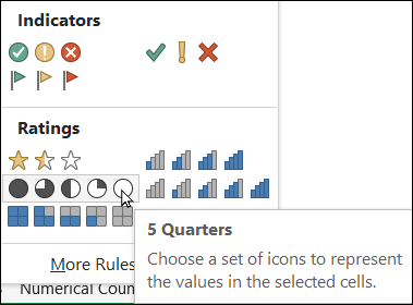
• In the pop-up menu, in the Ratings section, click on the Harvey Balls (5 Quarters icon set)

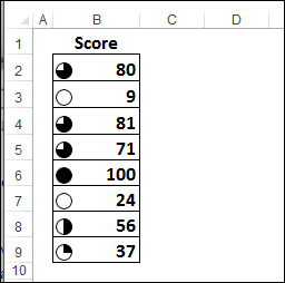
On the worksheet, the selected cells will show Harvey Balls icons, in black and white, based on the cell values.

• The cell with the highest number has a filled black circle
• The cell with the lowest number has an empty circle shape

Add Background Colour

If you’d like a splash of colour with the Black and White Harvey balls, you can add another conditional formatting rule to the cells.

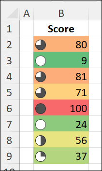
This time, use one of the Colour Scales, such as Red, Yellow, Green, like I did in the screen shot below.

Now, the cell with the highest number has a filled black Harvey ball, with a red fill colour. The lowest number is in a green cell, with an empty Harvey ball.

Optional: Customize Harvey Balls

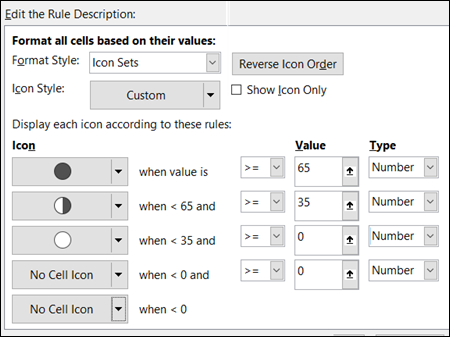
Instead of leaving the default Harvey Ball settings, with five different circles, you could customize the icon set, and use 3 balls, for a simpler look.

There are written steps on my Contextures site, and in the screen shot below, I changed the set to 3 balls, with number limits at 65, 35 and zero.

• Tip: You can use cell references for the values, instead of typing the numbers into the Rule Description.

Create Coloured Harvey Ball Icons

One way to overcome the black and white limitation with built-in Icon Sets, is to create your own icon set. I showed one way to do this last year, and you can see the details here.

Last week, Jim McGarity sent me a sample file with his version of icon sets, based on custom number formats and conditional conditional. That’s a great idea, Jim, and thanks for sharing it!

Steps to Create Custom Icons

There are 3 main steps in Jim’s technique to create Harvey balls in red, yellow and green.

1. Build a lookup table with scores and symbols
2. Create custom number formats with symbols
3. Apply conditional formatting rules

The details for each step are in the sections below.

1) Build a Lookup Table

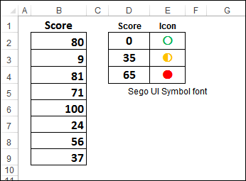
The first step is to build a small lookup table on the worksheet. The table has two columns:

• the number at which each level starts
• the Harvey Ball symbol for each level.

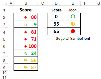
In the screen shot below, the lookup table is in cells D2:E4

Set Up the Table

To set up the lookup table, follow these steps:

• In D2:D4, type the minimum score for each level —  0, 35 and 65
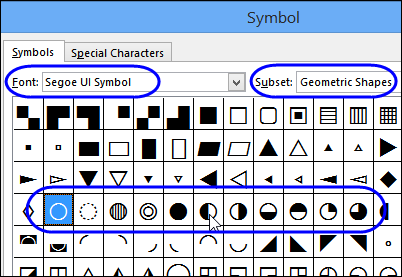
• In cells E2:E4, use Excel’s Insert Symbols feature to enter the empty circle, half-filled circle, and filled circle, from the Segoe UI Symbol font.
• (Optional) Change the font colour for each symbol, as shown in the screen shot above.

NOTE: The symbols are in the lookup table for reference only

2) Create Custom Number Formats

The next step is to create a number format for each symbol. These number formats will be used for conditional formatting later.

• Note: The number formats, shown below, use the ? (question mark) character, which is a spacer. That will make the numbers line up correctly on the worksheet. Visit the Microsoft website for more information on custom number formatting.

Copy First Symbol

• First, in the lookup table, select the cell with the empty circle symbol
• In the formula bar, select the icon, and press Ctrl + C, to copy it
• Press Enter, to exit the Formula Bar

Create First Number Format

• Next, select an empty cell on the worksheet
• Press the keyboard shortcut, Ctrl + 1, to open the Format Cells window.
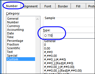
• Click the Number tab, and at the left, click the Custom category
• Clear out any text in the Type box
• Press Ctrl + V, to paste the symbol
• Next, type a space, then two question marks, and a zero:
  •   ○ ??0
• Click OK, to complete the number format

Make 2 More

• Next, repeat the steps, to create custom number formats for the other two symbols.

3) Apply the Conditional Formatting

The final step is to apply the conditional formatting to the column of Scores.

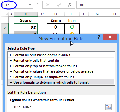
• To begin, select all the cells with scores – cells B2:B9 in this example
• On the Ribbon’s Home tab, click Conditional Formatting, then click New Rule
• Click Use a Formula to Determine Which Cells to Format
• For the formula, enter:   =B2>=$D$2
  • TIP: Make sure that the first reference is to the active cell – B2 in this example

 

• Click the Format button
• On the Number tab, select the custom format that you created earlier:
  • – ○ ??0
• Next, go to the Font tab
• Select Green as the font colour, then click OK.
• The preview will show the formatting, with the empty circle icon.

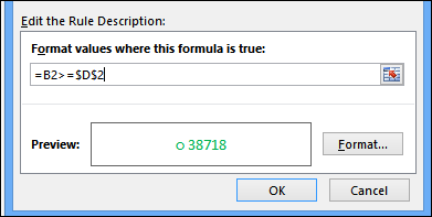
• Click OK, twice, to close the Conditional Formatting windows.

Repeat the steps for the other two symbols, then close the Conditional Formatting window.

The Completed Formatting

After you’ve applied the formatting, the icons will appear to the left of the number in column B, separated by a space.

Because the custom number formats used the question mark characters, the digits line up correctly.

• The 9, in cell B3, is at the far right of the cell
• It lines up with the final digit in the 100, in cell B6.

Download the Sample File

To download the sample file, go to the Conditional Formatting Examples page on my Contextures website.
This example is in the first download file, Conditional Formatting Basics, and it’s on the ColorIconsNum sheet.

Video: Conditional Formatting – Data Bars

Another way to show numbers visually, is with conditional formatting data bars. At a glance, you can see which cells have the largest and smallest numbers.

This short video shows how to set up Excel Data Bars, and change their default settings.

Related Articles

Create Your Own Excel Icon Set

Customize Excel Conditional Formatting Icons

Create Conditional Formatting Icons in Excel

________________