Highlight Upcoming Employee Service Anniversaries

Here at Contextures, there aren’t very many employees to keep track of. There’s just me, and I always remember my hire date anniversary, and take myself out for a nice lunch. However, you might have more people on your employee list, and you can use Excel to highlight upcoming employee service anniversaries.

Employee Service Anniversaries

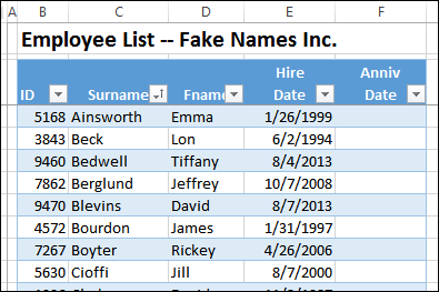
In the Excel Table shown below – filled with fake names and hire dates – there are 48 employees. That’s way too many people to manage, without some help!

I’ll add a formula to calculate each person’s anniversary date, based on their hire date. Then, I’ll highlight the rows which have upcoming anniversaries.

Enter the Current Year

To get the anniversary date for each person, we’ll create a date with the current year, and the month and day from the hire date. I’ve entered the year in a cell at the top of the sheet, and named that cell – CurrYear.

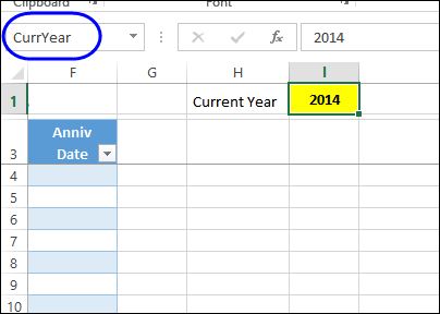
You could use a formula to get the year from the current date, but I like to type it on the worksheet. That way, it can be controlled at year end, if you’re finishing up some reports from the previous year, or getting a head start on next year’s reports.

Calculate the Anniversary Date

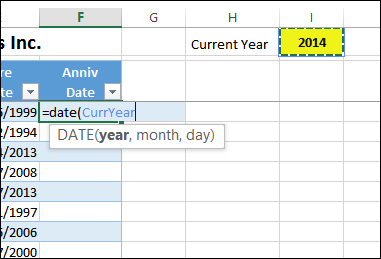
Next, I’ll add a formula in column F, to calculate the anniversary dates. I’ll use the DATE function, which has Year, Month and Day as its arguments. To get the year, click on the CurrYear cell, then type a comma separator.

=DATE(CurrYear,

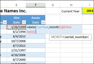
Next, use the MONTH function to extract the month from the Hire date. Because the data is in a formatted Excel Table, the field name, instead of a cell reference, is shown when I click on the Hire Date cell:

=DATE(CurrYear,MONTH([@[Hire Date]]),

Finally, use the DAY function to extract the day from the Hire date, then add a closing bracket for the DATE function. Again, the field name, instead of a cell reference, is shown when I click on the Hire Date cell:

=DATE(CurrYear,MONTH([@[Hire Date]]),DAY([@[Hire Date]]))

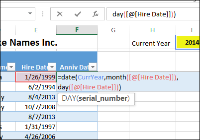
Press the Enter key, and the formula should fill down to the last row in the table.

Named Ranges for Date Range

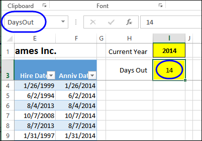
In the worksheet, we’ll use conditional formatting to highlight the upcoming anniversary dates. Instead of hard coding the number of days in the upcoming date range, we’ll add a named range – DaysOut – at the top of the sheet.

In the screen shot below, cell I3 has been named as DaysOut, and I entered 14 as the number of days.

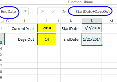
Next, we’ll add named ranges – StartDate and EndDate – at the top of the sheet, to show which date range is highlighted.

In the screen shot below, cell L1 – StartDate – contains a formula to calculate the current date: =TODAY()

Cell L3 – EndDate – add the specified number of days to the current date: =StartDate + DaysOut

Add the Highlighting

To add the conditional formatting,

• Select all the cells with employee data, but not the headings — cells B4:F51 in this example.
• Check the sheet to see which cell is active, because you’ll refer to that cell in the conditional formatting formula. In this example, cell B4 is active.
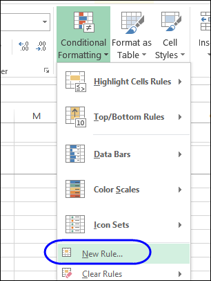
• On the Excel Ribbon’s Home tab, click Conditional Formatting, then click New Rule.

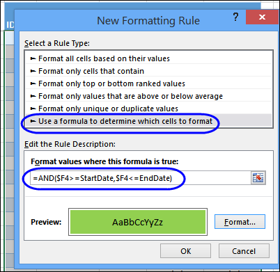
• In the New Rule window, at the top, click ‘Use a formula to determine which cells to format’
• Click in the Formula box, where you’ll add a rule that checks the anniversary date, to see if it is between the StartDate and EndDate. We’ll use the AND function to check both dates, and use a mixed reference to the anniversary date in the active row, locking the column, but not the row:
  =AND($F4>=StartDate,$F4<=EndDate)
• Click the Format button, and select a colour to highlight the upcoming anniversaries – I selected bright green.
• Click OK, to apply the formatting

The rows with anniversary dates that fall between the StartDate and EndDate are highlighted in green.

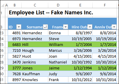
You can change the number of days, to change what is highlighted. For example, increase it to 30 days, and more rows might be highlighted.

Download the Sample File

To experiment with the conditional formatting, you can download the sample file from this tutorial. Go to the Sample files pages my Contextures website, and look for CF005 – Highlight Employee Hire Date Anniversaries. The zipped file is in xlsx format, and does not contain any macros.

___________________