With Excel’s conditional formatting, you can highlight cells based on specific rules. There are some built-in rules available, and you can use formulas to create your own formatting rules.
Highlight Duplicates
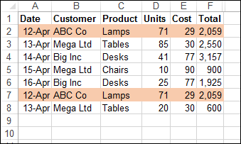
In this example, we want highlight duplicate records in a table. There is a built-in rule for highlighting duplicate values in a single column, but nothing that will check an entire row.
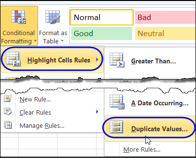
So, we’ll create our own rule, and it will require a new column on the worksheet, before we add the conditional formatting.
Concatenate the Data
In the sample data, there are two identical rows, and these should be highlighted after we apply our conditional formatting.
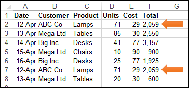
The first step is to use the CONCATENATE function to combine all the data into one cell in each row.
Add a new heading in cell G1 – AllData – and in cell G2, enter this formula, to combine the data from all the cells in that row.
=CONCATENATE(A2,B2,C2,D2,E2,F2)
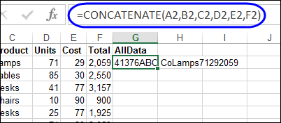
Next, copy the formula down to the last row of data.
Apply the Conditional Formatting
Then, a conditional formatting rule is set, to color the rows that are duplicate records. We’ll use the COUNTIF function to check for duplicates in the AllData column.
=COUNTIF($G$2:$G$8,$G2)>1
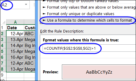
If there is more than one instance of a data combination, that indicates a duplicate row, and the cells in columns A:F will be coloured. The two rows with duplicate records are highlighted, so our conditional formatting formula worked!
Download the Sample File
For detailed instructions, and to download the sample file, please visit my Contextures website: Highlight Duplicate Records in a List
Watch the Video
To see the steps for setting up the conditional formatting, watch this short video.
_________________________

Cool!
What’s also cool about tables is that you can filter by color. So using a bit of VBA, you can then filter to show only duplicate rows, and then do something with them.
i need your help.i want to edit numbers within an excel cell.how can i do it?.when i hightligght’em and click outside the color’s gone.thanks a lot.
One very rare bug that may happen with this is if the data you have in two columns, when concatenated, looks the same. For example:
Col A   Col B   Concatenated

123     456     123456

1234    56      123456
This will show the rows above as duplicate when they are not.
@John, yes, if that’s a possibility you could put separator characters into the CONCATENATE formula.
On the subject of delimiters, you can’t beat the pipe character | (Shift + \)
Great Tutorial. But is there any way to highlight only a single instance of duplicate records? I mean if I could do so then it would be easier to just sort out the highlighted records and later delete them.
@Ankit Mac, if you only want to highlight the duplicate records, and not the first instance of a duplicated record, use this formula: =COUNTIF($G$2:$G2,$G2)>1
That checks the rows down to the current row for duplicates, so for the first instance, the count would be 1, and that row wouldn’t be highlighted.
I’m working on a project where I need to find records where certain fields are close matches. For example in the Company field one entry may be “SC Johnson Wax” and another “S.C. Johnson Wax” or “S C Johnson Wax”. Another would be where someone has misspelled a word so maybe they typed “Johnston” instead of “Johnson”. These are all things that stick out to the human eye but how to look for them programmatically?
This probably requires VBA. This thread will probably help, Rick:
http://www.mrexcel.com/forum/excel-questions/195635-fuzzy-matching-new-version-plus-explanation.html
@Rick,
Trying looking at using multiple wildcards, such as:
=COUNTIF(A1,”*s*c*john*wax*”)
This will get you a hit on most entries, but of course if the user leaves out the word “wax”, it won’t work.
@Rick
I had to do something similar, and used VBA. Depending on your application, you might try something like this:
http://en.wikipedia.org/wiki/Damerau%E2%80%93Levenshtein_distance
It has sample code written in C#, but I was able to convert this to VBA without too much trouble and use it very effectively.
My application was to select the correct employee (from an employee roster) even if the input name was spelled incorrectly.
Here is the code I came up with:
Public Function iDLD_EditDistance(ByVal sSource As Variant, ByVal sTarget As Variant) As Integer
””””””””””””””””””””””””””””””””
‘ Comments: Determines the Damerau–Levenshtein distance
‘ (Edit Distance) of two strings. More information
‘ can be found at:
‘ http://en.wikipedia.org/wiki/Damerau%E2%80%93Levenshtein_distance
‘
‘ Arguments: sSource – Source String
‘ sTarget – Target String
‘
‘ Returns: Integer – This should be an integer value used
‘ by calling routine to determine a matching
‘ string based on lowest edit distance
‘
‘ ————————————————————-
‘
‘
Dim m As Integer, n As Integer
Dim i As Integer, j As Integer
Dim i1 As Integer, j1 As Integer
Dim xc As Integer
Dim INF As Integer
Dim DB As Integer
Dim H()
Dim sd()
Dim sdlen As Long
Dim tsd, tchr, tchrS, tchrT As String
‘ Quick check to resolve 0 lenthg stings
If Len(sSource) = 0 Then
iDLD_EditDistance = Len(sTarget)
Exit Function
Else
If Len(sTarget) = 0 Then
iDLD_EditDistance = Len(sSource)
Exit Function
End If
End If
‘ Prevent inappropriately high Edit Distance values with short source strings.
‘ Otherwise, the Edit Distance for a string like “Weinb” would actually be smaller with “Way”
‘ rather than “Weinbrenner”, given a false ‘match’. It will also speed things up.
sTarget = Left(sTarget, Len(sSource) + 1) ‘ note that if Len(sSource) + 1 > Len(sTarget) then it will return the whole string
‘ Remove Capital letters
sSource = LCase(sSource)
sTarget = LCase(sTarget)
‘ Initialize Variables
m = Len(sSource)
n = Len(sTarget)
ReDim H(m + 2, n + 2)
INF = m + n
‘Initialize Matrix
H(0, 0) = INF
For i = 0 To m
H(i + 1, 1) = i
H(i + 1, 0) = INF
Next i
For i = 0 To n
H(1, i + 1) = i
H(0, i + 1) = INF
Next i
‘Initialize sd array
sdlen = 1 ‘ Initialize sd with first char using tsd
tsd = Mid(sSource, 1, 1) ‘ Enter first char of sSource into tsd
For i = 2 To m ‘ pick up iteration with 2nd char of sSource
tchr = Mid(sSource, i, 1)
If InStr(1, tsd, tchr) = 0 Then ‘ If the current Char is not in tsd then add it
sdlen = sdlen + 1
tsd = tsd & tchr
End If
Next i
For j = 1 To n ‘ Now do same for chars from sTarget
tchr = Mid(sTarget, j, 1)
If InStr(1, tsd, tchr) = 0 Then
sdlen = sdlen + 1
tsd = tsd & tchr
End If
Next j
ReDim sd(1 To Len(tsd), 1 To 2) ‘ ReDim sd() to actual deminsions
For i = 1 To sdlen ‘ Move tsd into sd()
sd(i, 1) = Mid(tsd, i, 1)
sd(i, 2) = 0
Next i
‘Begin processing strings
‘ Not really sure how it all works, but it does! 😀
‘ It uses a matrix, H(), in conjuction with sd()
‘ By flood filling the matrix, it will determine Edit Distance
For i = 1 To m
DB = 0
For j = 1 To n
For xc = 1 To sdlen
tsd = sd(xc, 1)
tchr = Mid(sTarget, j, 1)
If tsd = tchr Then
i1 = sd(xc, 2)
Exit For
End If
Next xc
j1 = DB
tchrT = Mid(sTarget, j, 1)
tchrS = Mid(sSource, i, 1)
If tchrS = tchrT Then ‘ Filling matrix with new value
H(i + 1, j + 1) = H(i, j) ‘ If = then previous low value
DB = j
Else
H(i + 1, j + 1) = H(i, j) + 1 ‘ if then Min of adjacent matrix cells
If H(i + 1, j + 1) > H(i + 1, j) + 1 Then H(i + 1, j + 1) = H(i + 1, j) + 1
If H(i + 1, j + 1) > H(i, j + 1) + 1 Then H(i + 1, j + 1) = H(i, j + 1) + 1
End If
If H(i + 1, j + 1) > H(i1, j1) + (i – i1 – 1) + 1 + (j – j1 – 1) Then ‘ Magic formula that is used for the matrix
H(i + 1, j + 1) = H(i1, j1) + (i – i1 – 1) + 1 + (j – j1 – 1) ‘ in the case of transposition
End If
Next j
For xc = 1 To sdlen ‘ More magic that helps with transpostion
tsd = sd(xc, 1)
tchr = Mid(sSource, i, 1)
If tsd = tchr Then
sd(xc, 2) = i
Exit For
End If
Next xc
Next i ‘ Matrix is now complete
iDLD_EditDistance = H(m + 1, n + 1)
End Function
Thanks, Steve.
Great to see your implementation.
But how this could be used to color-mark cells having a short DLD?
Hi Hugo,
I will say upfront that my suggestion was beyond the original post on using the Conditional Formatting feature. Because of that, the implementation in more complicated, and required the use of VBA. However, the question poised in the comment I replied to was a more complicated problem: “I need to find records where certain fields are close matches” How close is close enough? 🙂
First, here is the very basics of how I used it.
1) I started with a roster of names to check against. This is kept up to date with all persons possible correct names (employees in my case).
2) When a name is entered into a sheet (in designated name cells), the name is checked using a VBA call from a change event.
2.1) If there is an match with the roster, then do nothing
2.2) If no match, find the name with lowest edit distance by iterating through the roster. Replace entered text with the name found.
So, if I were to color mark cells with potential name matches, here is how I would do it.
Assume I’m starting with a known good name.
1) Parse the good name so there are no spaces or punctuation, just letters.
2) Iterate through the cells in question, parsing the cell contents to remove everything but the letters. At this point, things can be done to skip the cell of it has certain features. i.e. empty, only numbers, etc.
2.1) If there is an exact match, change the color of the cell
2.2) If not, find the edit distance. Change the color of any name that is within a certain of edit distance. This is where things can get fuzzy. There could be a weighted set of criteria. Edit Distance, number of letters, first and last letters the same, etc. Each of these criteria can be used to help produce more accurate results.
The nature of the problem is such that there will likely to be some false positives (cells with names that are highlighted that really aren’t matches) and some missed matches. I would think in this case the false positives would be preferred over missing a name that should be highlighted, but wasn’t. In the end, the person looking at the results will have to verify that any name highlighted is a correct ‘close match.’
Thanx, Steve.
When operating only one name at a time, then your approach will work perfectly.
Would be fine to have a solution showing the minimum of DLD distances of a name in line to all the others.
When having this, you can mark all the lines showing a very low DLD value, so indicating a possible doubled name.
No idea how to implement this.
I am curious as to how you could assign different colors to different sets of duplicates.
You can avoid the need for concatenation if you use the COUNTIFS function instead of the COUNTIF function:
=COUNTIFS($A$2:$A$8,A2,$B$2:$B$8,B2,$C$2:$C$8,C2,$D$2:$D$8,D2,$E$2:$E$8,E2,$F$2:$F$8,F2,$G$2:$G$8,G2)
This will look at all of the values in the row and count how many other rows have the same set of values.
You could then use a modified version of this to create your conditional formatting rule without the need to create a separate column in the spreadsheet to count the duplicates:
=COUNTIFS($A$2:$A$8,A2,$B$2:$B$8,B2,$C$2:$C$8,C2,$D$2:$D$8,D2,$E$2:$E$8,E2,$F$2:$F$8,F2,$G$2:$G$8,G2)>1
You can read more about this approach here: http://fiveminutelessons.com/learn-microsoft-excel/find-duplicate-rows-excel-across-multiple-columns
David
I created a mock set of columns (Last name, First name) to test why Conditional formatting is not working for me on my real data. I used the MATCH formula and found an error (extra space after a , ) It resulted in one False and I could see the extra space. But it did not find another that had a , after “Last name”. My columns had one that needed be concatenated. Conditional formatting did yield duplicates.Also is there a way to request the duplicates to be put into a new column?
thanks in advance,
Maggie
I have a 2-column list with “telephone-number” in one column and “comment” in the other (the “comment” column may be empty).
How can I identify and remove duplicate telephone-numbers even if the comments are different?
The “Remove duplicates” function only removes duplicate telephone-numbers if the respective comments are identical.
Example:
999999999;Home
999999999;Ann
999999999;Home
Excel only identifies the first and the third row as duplicates.
If I select the first column only, duplicate telephone numbers get removed, however, the comments no longer match as none got removed.
Thanks for helping
Bruno
Select both columns, and in the Remove Duplicates dialog box, remove the check mark from the Comment heading.
There is a video here that shows the steps:
http://blog.contextures.com/archives/2013/11/26/remove-duplicates-in-excel-2013-list/
Hi,
i have a list of employee names which has a the full name(s) of the employees now the requirement is we need a separate fields for First name and last name what formula i can use to do this?
Can i delete back the “Concenated” column and leaving the duplicates data only???
I have a data set which requires an exact formula due to case sensitivity. What would I use instead of =COUNTIF($G$2:$G$8,$G2)>1
Thank you all for sharing your knowledge, I appreciate it!