When you create a list in Excel, do you automatically convert that list to a formatted table?
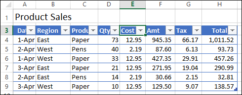
If not, you’re missing out on one of Excel’s best features.
- Formatted tables are easy to set up, and make it easy to sort, filter, format, and expand your list.
- You can refer to the table’s fields in your formulas, and the reference will adjust automatically, if you add or remove data.
Set Up Your Data
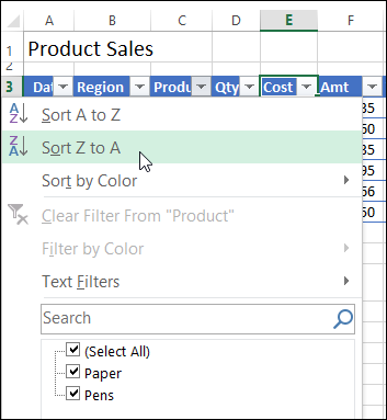
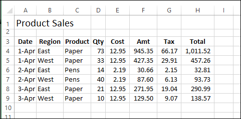
There are a few things to check, before you turn your data list into a table. For example:
- Add a heading in each data column
- Leave blank rows and columns around the list
- Don’t leave blank rows or columns within the list
Create the Table
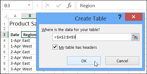
Once the data is set up, select any cell in the list, and click the Table command on the Ribbon’s Insert tab. When the Create Table window opens, check that the range is correct, and check the box for “My table has headers”.
Name Your Table
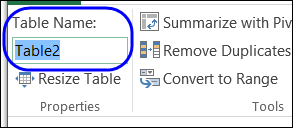
After you create the table, change its name from the default “Table1” to something meaningful, such as “Orders”. This is especially important if you’re going to have more than one table in the workbook.
Just type over the old name in the Table Name box on the Ribbon’s Design tab.
More Table Tips
For more tips on working with tables, visit the Excel Tables page on my Contextures website.
Watch the Video
If you haven’t made a formatted table before, watch this video, to see the steps.
The video is also on the Excel Tables page on my Contextures website.
__________________

Here’s one that’s an extention of the second bullet point, but worth explicitly stating:
You can use them as a data source for a pivot table, and the pivot will automatically take into account any changes in the table. NO MORE USING THE “CHANGE DATA SOURCE” FUNCTIONALITY FOR PIVOTS!!
Sorry for shouting 😉
Also worth giving a shout-out to my favourite Excel shortcut…Ctrl + T
@Jeff Thanks for the shortcut reminder. And Ctrl+L works too — I sometimes hit that accidentally, when trying to use Ctrl+; for the date.
And what isn’t widely known: even if you use “normal” cell references in formulas that point to a table’s columns, those formulas will be adjusted when the table expands or contracts. So also no more entire column references in VLOOKUPS.
@Jan Karel — thanks for mentioning that feature. It’s useful when you don’t want to use the field names in a formula.
Another point to note about Table references is that they point to the Table no matter where you move the table in the workbook, and no matter what data you add or remove around it.
That is damn hard to accomplish using formulas alone, because most dynamic formulas also have hard references to the rows/columns where your data sits; and/or use COUNTA or similar which can be ‘upset’ if the user adds more data between the table and the top/side of the spreadsheet.
Which raises a good question…why don’t Pivots have something similar? GETPIVOTDATA is a far cry from Table references.
Aside: I had a crack today at writing a non-volatile formula that works the same as table references i.e. is completely dynamic, doesn’t care about extra data being added around the table, and allows the table to be moved anywhere. It has just the one reference to the data…a named range called TopLeft:
=TopLeft:INDEX(Sheet1!$1:$1048576,ROW(TopLeft)+MATCH(1,INDEX(--(ISBLANK(TopLeft:INDEX(INDEX(Sheet1!$1:$1048576,,COLUMN(TopLeft)),COUNTA(INDEX(Sheet1!$1:$1048576,,COLUMN(TopLeft)))+ROW(TopLeft)))*ROW(TopLeft:INDEX(INDEX(Sheet1!$1:$1048576,,COLUMN(TopLeft)),COUNTA(INDEX(Sheet1!$1:$1048576,,COLUMN(TopLeft)))+ROW(TopLeft)))>ROW(TopLeft)),0,0),0)-2,COLUMN(TopLeft)+MATCH(1,INDEX(--(ISBLANK(TopLeft:INDEX(INDEX(Sheet1!$1:$1048576,ROW(TopLeft),),COUNTA(INDEX(Sheet1!$1:$1048576,ROW(TopLeft),))+COLUMN(TopLeft)))*COLUMN(TopLeft:INDEX(INDEX(Sheet1!$1:$1048576,ROW(TopLeft),),COUNTA(INDEX(Sheet1!$1:$1048576,ROW(TopLeft),))+COLUMN(TopLeft)))>COLUMN(TopLeft)),0,0),0)-2)It ain’t pretty. Thank goodness for tables, I say.