One of my favourite Excel features is a data validation drop down list. In just a couple of minutes, you can make a list of items, then make that list appear in a worksheet cell. It’s like magic!
The drop down lists make it much easier to enter data, and they help prevent typos, or invalid entries.
Note: The DVSP tool is a free version of the popular DVMSP tool that I sold for several years. In the videos, screen shots and written steps, you might see “DVMSP”, instead of “DVSP”.
Video: How to Use DVSP Setup File
Next, you can watch this video to see the DVSP setup file steps, and there are written instructions in the Setup file.
Excel Skills Needed
To use the DVSP tool, you will need the following Excel skills, to get your file ready:
create a named range (for the list of items) — there are instructions and a video here: Create a Named Range
create drop down list(s) on the worksheet, based on a named range — there are instructions and a video here: Create a Drop Down List
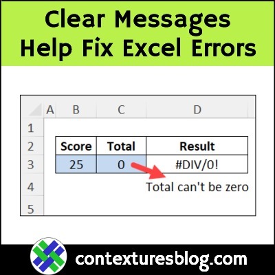
Did you know that you can use the Excel ERROR.TYPE function to identify specific types of errors on a worksheet? And after the error type is identified, you can use that information to provide help with error troubleshooting.
There’s a short video below, that shows an example, and there’s a list of the Excel error values that this function can identify.
I add lots of screen shots to my Excel tutorials, so it’s easier to follow the steps. And if I’m explaining a formula, it’s helpful to show that on the worksheet too.
However, some Excel formulas can get pretty long, and I found a way to fix that problem! You can see all the solutions that I tried, or skip to the end, to see the final solution.
Do you use Excel to help with all of your holiday planning? It’s a great tool for shopping lists, holiday budgets, dinner preparation, and even holiday games!
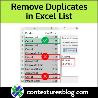
There’s a built-in tool in Microsoft Excel that makes it easy to remove all the duplicate values from a list. You can remove duplicates based on the items in one column, or multiple columns.
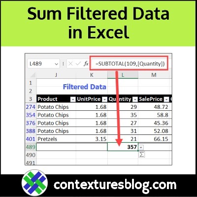
When an Excel list is filtered, how can you show a total sum or count for numbers in the visible rows only? There are two Excel functions for that task — SUBTOTAL (all Excel versions) and AGGREGATE (Excel 2010 and later). See how these functions work, and decide which one to use.
There’s a video further down the page, where I show both functions, along with the Excel SUM function. That might help you decide which function will work best for you.
Old Versions of Excel: If there’s any chance that you’ll have to share the file with someone who’s using Excel 2007 or earlier, go with the SUBTOTAL function. Yes, those are really old versions of Excel, but some people haven’t upgraded.
Easy to Use: It’s easy to insert the SUBTOTAL function below a filtered list:
Select the blank cell immediately below the column of numbers
On the Excel Ribbon’s Home tab, click the AutoSum button.
Excel automatically inserts a SUBTOTAL formula for you, with the Sum function (9) selected.
NOTE: In newer versions of Excel, function 109 is automatically selected, so change that to 9, if you need compatibility with older Excel versions
Excel automatically inserts SUBTOTAL formula
Excel AGGREGATE Function
If you don’t have to share the Excel file with anyone who’s using Excel 2007 or earlier, I’d recommend using the AGGREGATE function.
Here are a couple of reasons to choose AGGREGATE:
It has 19 functions, compared to the 11 functions in old versions of SUBTOTAL
There are 8 options for what to ignore, compared to the 2 options in SUBTOTAL
AGGREGATE function has 19 functions
Video: Sum Filtered Excel Data
This short video shows how to sum filtered numbers in Excel, with the AGGREGATE function, or the Excel SUBTOTAL function.
You’ll also see the differences between those two functions, and how they compare to the SUM function.
Make it easy to enter valid data in an Excel workbook. Choose “Fastener” in one combo box drop down. The next combo box shows a list of fastener parts, with part ID and part name.
This video shows how to use this simple data entry tool, and you’ll get a peek behind the scenes, on how it works.
Video Timeline
Here’s the video timeline, and the full video transcript is at the end of this post:
0:00 UserForm Demo
0:53 Lookup Lists Sheet
1:25 See How Macro Works
1:48 Named Range for Parts List
2:02 UserForm Macro Code
Dependent Combo Box Drop Downs
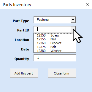
In the screen shot below, you can see the Excel UserForm from my video.
From the Part Type combo box drop down list, I selected Fastener
That affects the Part ID combo box, which is dependent on the Part Type selection
Instead of showing all the parts, the Part ID drop down only shows a list of Fastener parts.
When you select a part, only its Part ID is stored in the combo box
That makes it quick and easy to enter data.
Parts Inventory UserForm with Dependent Combo Box
Add to Parts Inventory
After you fill in the Parts Inventory boxes, click the Add This Part button.
That button runs Excel VBA code, which puts your data into a worksheet Excel table, for storage.
Later, you can filter that table, to find specific entries. Or, build a pivot table from the data, to get an inventory summary.
Video Transcript: Excel UserForm With Dependent Combo Boxes
Custom Tab on Excel Ribbon
This workbook is set up so you can enter parts data, using an Excel UserForm.
On the Ribbon, there’s a special tab for this workbook, called DB macros.
If you click that, you’ll see the buttons along the Ribbon, and to open the form you click Data Entry Form.
Excel UserForm Opens
In the UserForm, you can select from the drop-down list.
It automatically fills in the current date, and a quantity of 1, and you can change those fields if you need to.
The first field is a Part Type, and the second is a Part ID
Right now, there’s nothing showing this Part ID list, because first you have to choose a part type.
There are 2 types, so we’ll select Fastener
Once I select that, then there’s a list of the fasteners
Select one of those, and its part number shows up here
Then you can select a location, and then add that part.
Add Part Order
Once you click Add Part, it clears out the top 3 combo boxes, and resets the date and quantity.
To see how this works, I’m going to go to a different sheet in this workbook, which is Lookup Lists.
See Lists Sheet
And here’s a list of all the parts with their ID, which category they’re in, and then a
description of the part.
We also have lists for the location. That’s another combo box, and the categories — we’ve got two categories.
Over here, there’s a setup for a filter. Whenever you select a part category, that name goes into this cell, and it’s a criteria range for an Advanced filter.
See How Macro Works
I’ll reopen the data entry form.
When I select a part type, fastener, nothing happens right away.
But when I leave that combo box, I’ll click in Part ID.
Now you can see that it’s put fastener into the criteria range
It ran an advanced filter, and gave me a list of all the fastener parts.
I’ll click the part ID, and I can now see that list that’s on the worksheet.
I’m going to close the form again, and this works with names.
Named Range for Parts List
Whenever it creates this list, it gives it a name. You can see here: PartSelList
That is used for the combo box for the parts
To see the code, we can go into Visual Basic, and here’s the UserForm
UserForm Macro Code
The part type, if I double click on that, you can see that after the update, this code runs.
It clears out any existing value in the part drop down
Then it sets the row source, which is that named range
It sets it to nothing, so that combo part won’t have any items in it
Then it puts a current category value into the criteria range, runs the filter, and it redefines that list
So if it’s longer or shorter, it adjusts that, and then it sets the part combo box to have
that range as its source.
In some workbooks, you might need to block duplicate entries in a column. For example, we don’t want 2 employees to have the same ID number. See how to set up a custom rule for that, with data validation. And keep reading, to see why COUNTIF can cause problems for you.