Highlight Upcoming Dates in Excel

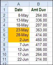
Do you use Excel to keep track of upcoming payments, or other dates? To make that list more helpful, you can highlight upcoming dates in Excel. In this example, we’ll highlight dates if they’re within the next couple of weeks.

Compare Cells With a Simple Formula

With Excel’s conditional formatting feature, you can highlight cells that have a specific value, or that meet other conditions. Recently, we used conditional formatting to show where a new date starts, in a list of dates.

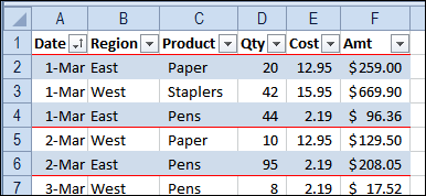
That red border was created if the date in column A was different from the date in the cell above. A simple formula checked the two cells, and created the top border if the cells were not equal:

=$A2 <> $A1

Calculate the Date Difference

In today’s example, we want to highlight the cells where the date is between today and two weeks from today. We’ll need a formula that does more than compare two cell.

First, the formula will have to calculate how many days are between today and the date in the cell. To do this for cell A2, the formula is:

=$A2 – TODAY()

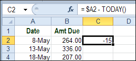
The result is –15, so that date was 15 days ago.

Check a Date Range

The next step is to see if the date difference is within the range that we want to highlight. That range goes from today, which is zero days difference, to the date two weeks from now, which is +14 days difference.

To check the date range with a worksheet formula, we’d use the AND function, combined with the days difference formulas:

=AND($A2-TODAY()>=0,$A2-TODAY()<=14)

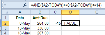
If the date difference is greater than or equal to zero, AND the date difference is less than or equal to 14, the result is TRUE. Those are the dates that we want to highlight.

Create the Conditional Formatting

To highlight the cells in the date range, we can use the same formula.

1. Select date cells – cells A2: A11 in this example. Cell A2 is the active cell.
2. On the Excel Ribbon’s Home tab, click Conditional Formatting, then click New Rule
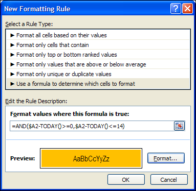
3. In the New Formatting Rule dialog box, click Use a Formula
4. In the formula box, enter this formula:
   =AND($A2-TODAY()>=0,$A2-TODAY()<=14)
5. Click the Format button.
6. Select formatting options (orange fill, in this example), click OK, twice, to close the dialog boxes.

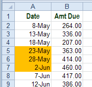
Dates Highlighted

Now, the dates in the two weeks upcoming are highlighted in orange.

Use a Cell Reference

To make the conditional formatting more flexible, you could use a cell reference in the formula, instead of typing the zero and 14.

For example, put your minimum and maximum days difference in worksheet cells, and name those cells. Here, the cells are named MinDays and MaxDays.

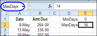
Then, change the conditional formatting formula to use those cell references:

=AND($A2-TODAY()>=MinDays,$A2-TODAY()<=MaxDays)

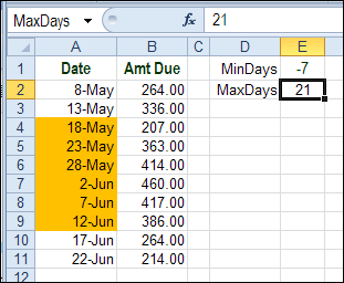
After changing the formula, you can change the days on the worksheet, and the conditional formatting will automatically adjust.

For example, change the MinDays to -7 and MaxDays to 21, and the date range goes from 1 week ago, to three weeks from now.

More Conditional Formatting Examples

You’ll find many more conditional formatting examples and tutorials on the Contextures website.
______________