To format a pivot table, you can select a specific section, such as one of the fields, or a grand total. When you point to a field heading, a black arrow will appear, if the Enable Selection setting is turned on.
Black Arrow Pointer
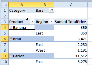
In the screen shot below, you can see the black arrow at the top of the Product field. Click in that spot, and all the Product item labels are selected.
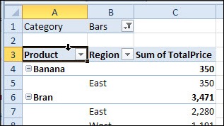
Click in that spot again, and the Product heading is selected, instead of the item labels.
Pivot Table Field Setting Quick Tip
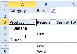
Instead of a single click on a heading cell, you can point to an outer field heading and double-click when the black arrow appears.
In the screen shot below, the black arrow is on the Bran product heading cell.
Note: This trick won’t work on an inner field, like Region, which has no other fields under it.
Open Field Settings
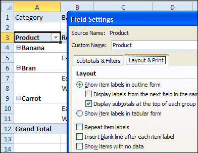
Double-click on the outer field heading, and the Field Settings dialog box opens.
In there, you can change the layout and other settings, and add or remove subtotals.
Right-Click Menu
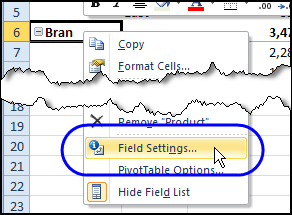
Another way to open the Field Settings dialog box is to right-click on an item, and click Field Settings in the popup menu. This works for both inner and outer fields in the pivot table.
I find the double-click shortcut to be quicker and easier – as long as you remember to point somewhere that the black arrow appears.
Watch the Pivot Table Selection Video
To see the steps for selecting section of an Excel Pivot Table, you can watch this short video tutorial.
_________________

0 thoughts on “Excel Pivot Table Selection Quick Tip”