Change Data Source for All Pivot Tables

If you want to change the data source for a single Excel Pivot Table, you can use a command on the Ribbon. If you want to change data source for all pivot tables in a workbook, you can use a macro, instead of making the changes manually.

Video: Change Pivot Table Data Source

In this video, you’ll see how to locate the pivot table data source,
then check that data source, to make sure it includes all the rows
and columns that you need. If needed, adjust the data source, to
include new rows or columns.

• NOTE: For a long term solution, use a named Excel table, as a data source. It will adjust automatically, if new rows are added.

To follow along with the video, you can download the sample file from the Pivot Table Source Data page on my Contextures site.

The full video transcript is at the end of this page.

Video Timeline

• 00:00 The Orders Pivot Table
• 00:21 Manually Check the Numbers
• 00:33 Find the Source Data
• 01:08 Change PivotTable Data Source Window
• 01:27 Fix the Data Source Range
• 01:57 Create a Dynamic Source
• 02:48 Create a Named Table
• 04:22 Use Dynamic Source for Pivot Table
• 04:56 Test the Dynamic Source
• 05:31 Conclusion

Change Data Source One Pivot Table

Follow these steps, to change the data source for a single pivot table.

• Select a cell in the pivot table that you want to change
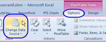
• On the Ribbon, under PivotTable Tools, click the Options tab
• Click the upper part of the Change Data Source command

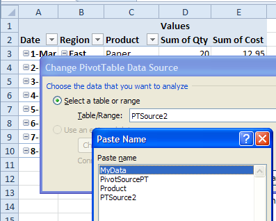
• When the Change PivotTable Data Source dialog box opens, press the F3 key on the keyboard, to open the Paste Name window.
• Click on the named range that you want to use, and click OK

• Click OK to close the Change PivotTable Data Source dialog box.

Change All the Pivot Tables in the Workbook

If you have several pivot tables in a workbook, and want to change all of them to a new data source, you can use a macro, instead of making the changes manually.

I’ve added a new page on the Contextures website – Excel Pivot Table Data Source – with sample code to update all the pivot tables.

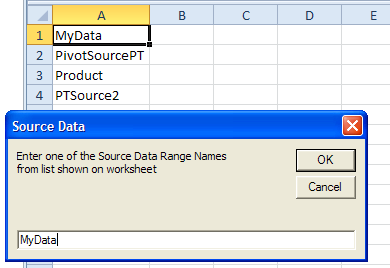
The macro adds a sheet to your active workbook, showing a list of the file’s named ranges. Then, the macro prompts you to enter one of those names, as the new data source for all the pivot tables.

____________

Video Transcript: Locate and Change Excel Pivot Table Data Source

In this video, you’ll see how to find the source data for a pivot table and fix that source data, if there’s a problem getting the new or changed data that you’ve entered. In this pivot table, I’m showing orders. One of the products we sell is paper, and I entered a new order, with 200 as the quantity, and it’s not showing up here.

If I right click and refresh, it keeps showing 20 and 10 so it’s not picking up that new record. I’m going to find the source data and see if there’s a problem.

To find the source data, I have the cell selected in the pivot table. Up on the Ribbon, I can see Pivot Table Tools, and I’m going to click Analyze. If you’re using Excel 2010, this would say Options.

I’ll click here, and here’s the Change Data Source. There’s also a drop down list, but it’s quicker to just click at the top of this.

That opens up the Change PivotTable Data Source window.

It’s showing that there’s a range selected, and I can see those little moving lines in the background, and we can see that one row is not included here.

It stops at row 9 and the new record that I put in is row 10. That’s where my 200 is, and it’s not being picked up.

To change this and fix the problem, I can adjust the range that’s included here. So I could click, just back space, and type 10, instead of 9.

Or I can select all of this and delete it.

Then on the worksheet, select the exact range that I want to use. Then click OK, and when I go back to the pivot table, instead of 20, it’s now showing 220, so it’s picking up the new data.

You could continue to adjust that range as you add new rows to the data source.

But a better solution is to create a dynamic source for your pivot table, which will adjust automatically, if you add new records.

It’s easy to do that, if you’ve got Excel 2007 or later. I’m going back to the Orders sheet.

This is just a list that’s typed on the worksheet. We’ve got column headings and a row for each order, but if I look up on the ribbon, there’s no extra tab at the top.

We’re going to create a named table. It will be a special feature, and when I select a cell, if it’s a named table, I’ll see another toolbar that I can use, to work with that table.

To create the table, it’s quick and easy. Just select a cell in your list and on the Ribbon click Insert, Table.

It does a very good job of detecting the range, but if it didn’t select all the cells, you can adjust what’s typed in here.

Make sure that the check mark is here for My Table Has Headers, and then click OK.

You’ll get a formatted table. I’ll just click on one cell.

I don’t usually like the formatting that it puts on the table at first, but you can go up to the Design tab, there’s that Table tab that is appeared now, and select something that’s simpler and easier to read.

The next thing you should do right away is change the name of the table. It will give a default name that ends with a number.

Just select that and I’m going to call this tbl, for table, tblOrders, and press Enter.

So now we have a table name, and I can see that name,

if I go to the Formulas tab, Name Manager.

And there’s a list of all the names in this workbook. So it makes it easy to spot this, if you have several tables in your workbook.

I’ll close this, and the next step will be to use our name, so going back to the Table Tools, we’re going to use this name, tblOrders, as our source for the pivot table.

I’m going to just click in here, and then Ctrl+ C to copy that name.

I’ll go back to my pivot table now. And then with a cell selected in the pivot table, I’ll go back to the Analyze tab, click Change Data Source, and here’s the current data source.

I’m going to use Ctrl+ V to paste what I copied as the table name. So it’s now going to use this dynamic range which will adjust as we add new records.

Click OK, and nothing looks different here, but I’m going to go and add another order.

Just copy what we have above, by using Ctrl and the double quote. I’ll put in 100, so now we should see 320, where we had 220 before.

Going back to Pivot Sales, it still says 220. I’ll refresh, and now we’ve got 320.

So I didn’t have to adjust the range of the pivot table source data. That adjusted automatically, because it’s a named table.

So if your pivot table data will change frequently, make sure you use a dynamic source, like a named Excel table, and it will adjust as you add or delete records.

For more Excel tips and tutorials, and to download the sample file for this video, please visit my Contextures website, at www.contextures.com