Last week, we used the Excel SUBTOTAL function to sum items in a filtered list, while ignoring the hidden rows. Now we’ll look at ways to use Subtotal and SumProduct with filter settings applied.
Subtotal Function
Here’s a screen shot of the SUBTOTAL function options, that we used last time.
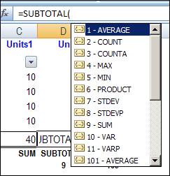
In the comments for that blog post, Sam mentioned that you can also use SUBTOTAL with functions like SUMPRODUCT, to do additional sums or counts, based on the visible data in a filtered table.
Sam sent me his sample Excel file, to show how he uses this technique.
Create Named Ranges
Sam’s workbook has a list with Product, Region and Amount fields. He created dynamic named ranges for the entries in each field, using INDEX and COUNTA.

Note: If you’re using Excel 2010 or Excel 2007, and a named table, you can use table references to create the names.

The SUMPRODUCT Function
With the a simple SUMPRODUCT function, you could sum the amounts for all the North region rows. This works well if the list is not filtered.
=SUMPRODUCT((Region=A2)*(Amt))
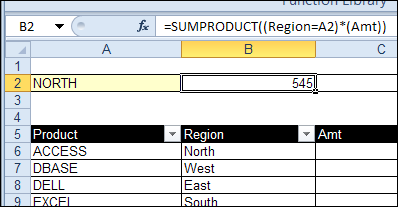
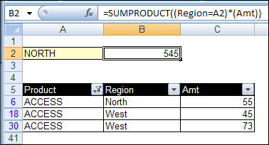
However, if the list is filtered, the total for North region still calculates as 545, even though only one amount, 55, is visible.
Another Named Range
To solve the problem, Sam created another named range, vAmt, that is based on the Amt range.
=SUBTOTAL(109,OFFSET(Amt,ROW(Amt)-ROW(‘1’!$C$6),,1,1))
The named range uses the SUBTOTAL function to return an array of the values, with zero showing if the row is hidden.
Use SUBTOTAL with SUMPRODUCT
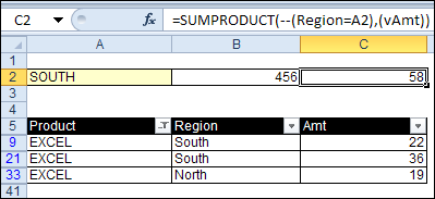
When the vAmt range is used in a SUMPRODUCT formula, it shows the total for only the visible rows.
In the screen shot below, the South region is selected, and the two visible amounts for that region are totaled correctly in cell C2
See the Formula Details
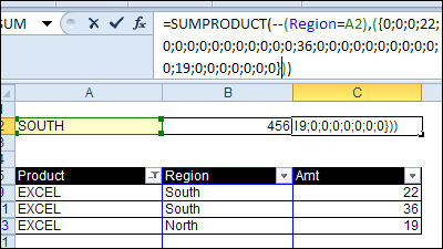
If you select the vAmt in the formula, and press the F9 key, you can see the effect of the SUBTOTAL function.
All the amounts show as zero, except for the three visible amounts — 22, 36 and 19.
Download the Sample File
For more formula examples, and to get Sam’s workbook and formulas, go to the Excel Filtered Rows – Count or Sum page, on my Contextures site.
In the Download section on that page, look for sample #4 – Sam’s Workbook. The zipped file is in Excel xls file format, and does not contain any macros.
___________________
Related Links

Another alternative to the above is to create a “visible flag” at source via a suitable SUBTOTAL calculation
Using Sam’s sample file:
D6:
=SUBTOTAL(3,$A6)
copied to remaining rows
We can then create a further Defined Name for this range – using Sam’s constructs:
Name: Vis
RefersTo: =Data!$D$6:INDEX(Data!$D$5:$D$65536,COUNTA(Data!$A$5:$A$65536))
note: use COUNTA of A for consistency
At this point our syntax is simplified such that our SUMPRODUCT becomes:
=SUMPRODUCT(–(Region=$A$2),Vis,Amt)
The above is also non-volatile.
Debra,
I have set up a list of items as a named range (Profit_centers), which I use to populate another named range(Selected_PF)using validation.
I have a series of sumproducts
(=SUMPRODUCT(Rev_Budget_QTD;–(Rev_Profit_Center=Selected_PF);(–(rev_Quarter=C$5&”-“&RIGHT($F$1;2))))
that work perfectly for each item in Profit_centers, when selected in selected_PF.
My problem is that I don’t know how to create a single item for Profit_centers (namely “All”) that, when selected, tells the sumproduct formulas to select all Profit_centers, instead of one.
any ideas?
as always, thanks for your help.
Martin
There is a site that provides the way to count the unique values in a column.
And there is a way is using the formula: =SUMPRODUCT(1/COUNTIF(List1, List1))
I am finding the way to combine the above-mentioned formula with Auto Filter function in Excel. Could you please help me?
Thanks
can you help about this:
i have found a way to ignores duplicated values in COUNTIF function this way
kind % Qutty 1/Qutty
a 50 2 1/2
a 20 2 1/2
b 10 3 1/3
b 70 3 1/3
b 5 3 1/3
d 80 1 1
c 10 1 1
f 65 1 1
so we have 5 kinds simply by a SUM function
but if i user a filter like >30% this will show a wrong answer
any help about a dynamic COUNTIF that ignores hidden rows?
@Sina, you could use a variation of the SUMPRODUCT formula, shown here:
http://www.contextures.com/xlFunctions04.html#Visible
Hi All
I have facing a problem in excel. I have to use countifs formula for some assignments.But I am not able to work because its not working in a filter mode. So how could i execute the same. Below is an example I need city wise count for the below criteria . >=85 & >5. Plz help
for an example :
>=85 >5
CITY CIRCLE EDGE IP Throughput (DL) TOTAL VOLUME( MB)
NON SHOWCASE ASSAM 126.92 48.33
NON SHOWCASE ASSAM 176.63 120.82
NON SHOWCASE ASSAM 144.94 38.77
GUWAHATI CITY ASSAM 80.26 128.1
GUWAHATI CITY ASSAM 122.71 45.35
GUWAHATI CITY ASSAM 90.22 74.86
JORHAT ASSAM 181.7 39.78
JORHAT ASSAM 145.58 45.04
JORHAT ASSAM 171.83 96.27
@Kalyan, there are instructions here for counting specific items in a filtered list:
http://www.contextures.com/xlFunctions04.html#Visible
I have hit a bit of a road block.
I need to calculate a weighted average for filtered rows. I am able to get the standard average using subtotal but cannot figure how to nest the sumtotal function into the subtotal one.
name Industry Population Q1
ABC Agro 331 4.61
DEF Tech 551 4.56
Normal average 4.58
Weighted average 4.57