Last Friday, there was an HLOOKUP example, and it used a dynamic lookup range — as rates were added to the lookup table, it automatically expanded to include them.
Today, we’ll take a closer look at that dynamic range, and see how the INDEX function is used to set the last cell in the range.
Count the Cells
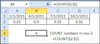
To find the last column for the INDEX function, you can use the COUNT function to count the rates that are entered in row 2.
=COUNT($2:$2)

Create a Cell Reference
The INDEX function can return a cell reference, based on a row number and column number in a reference.
Here are the arguments in the INDEX function syntax:
- INDEX(reference,row_num,column_num,area_num)
Count the Columns
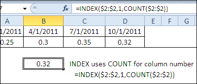
Using row 2 as the reference, the COUNT function can provide the column number. There is only 1 row in the reference, so 1 is used as the row number:
=INDEX($2:$2,1,COUNT($2:$2))

This formula creates a reference to cell D2, and its value is shown in cell B7.
Create the Dynamic Range
The same INDEX formula can be used in a defined name, to create a dynamic range.
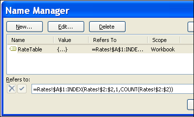
In the example shown below, the RateTable named range:
- starts in cell A1 on the Rates sheet
- ends in the cell reference created by the INDEX function.
Here is the formula used in the Name Manager:
- =Rates!$A$1:INDEX(Rates!$2:$2,1,COUNT(Rates!$2:$2))

If a rate is added or removed in row 2
- the COUNT function result will change,
- the INDEX function will return a different ending cell for the dynamic range.
Download the INDEX Dynamic Range File
To see the defined name and the INDEX examples, you can download the INDEX dynamic range sample file.
______________

How does INDEX compare with OFFSET for dynamically named ranges? I’ve used something like =OFFSET(A2,0,0,1,COUNT(2:2)) to set the range for a problem like this, but I’m always looking for better solutions (otherwise I wouldn’t subscribe to 20 Excel RSS feeds).
Is INDEX a better solution, or just a different one? Or is there a time for INDEX and a time for OFFSET when creating dynamic ranges?
Aha !!!! ExcelFF. Kind of Excel for Tweet Freaks. Love it.
@ David – I believe it’s a matter of calculation speed. OFFSET is volatile & will recalculate even if all you did was re-filter the darned sheet. If you’ve got a gazillion dynamic ranges this will make a BIG difference.
@ Debra – Once again, THANKYOUTHANKYOUTHANKYOU!
@David, I agree with Lynda — INDEX is non-volatile, and your workbook should perform better if you use it instead of OFFSET.
@Tony, thanks! Functions are your friends too. 😉
@Lynda, you’re welcome! And thanks for answering David’s question.
Yes, I forgot to consider the volatility. That would make the difference right there. Well, it looks like I’m a changed man – it’s INDEX for dynamic ranges from here on out. Thanks for the tip.
I believe all the dynamic ranges are volatile, so I don’t think they will be a performance benefit from using Index instead of Offset when creating dynamic ranges. However, they will be a better performance when you use
=SUM(A1:INDEX(A:A,C1) over =SUM(OFFSET(A1,,,C1,)).
Regards
There are two forms of the INDEX function: array and reference.
You mention the INDEX function can return a cell reference, yet show the syntax for the Array form, =INDEX(array,row_num,column_num), which only returns a value.
The INDEX function syntax for the Reference form is INDEX(reference, row_num, [column_num], [area_num]) which returns the reference of the cell at the intersection of the row_num and column_num. The Dynamic range you create is receiving a reference from the INDEX function using the Reference form of the function. Correct?
Deb,
Great post, as usual.
I used to go with COUNTA (which would count non-numerics) when doing this, but more recently I switched to MATCH.
So, for example, instead of:
=Rates!$A$1:INDEX(Rates!$2:$2,1,COUNT(Rates!$2:$2))
I would use:
=Rates!$A$1:INDEX(Rates!$2:$2,1,MATCH(10^200,Rates!$2:$2))
If the “last” value is expected to be text instead of numeric or a date:
=Rates!$A$1:INDEX(Rates!$2:$2,1,MATCH(“ZZZZZZZZZZZZ”,Rates!$2:$2))
In the dark days before Tables were available, I often used a dynamic range like this as the basis for a PivotTable, if the values in Col A were numeric/dates:
=Rates!$A$1:INDEX(Rates!$1:$65536,MATCH(10^200,Rates!$A:$A),MATCH(“ZZZZZZZZZZZZ”,Rates!$1:$1))
or if Column A had text:
=Rates!$A$1:INDEX(Rates!$1:$65536,MATCH(“ZZZZZZZZZZZZ”,Rates!$A:$A),MATCH(“ZZZZZZZZZZZZ”,Rates!$1:$1))
Patrick
@Gregory, thanks, I’ve corrected the syntax in the article.
Ha ha…Good post, but especially love the amusing add for Colonix at the top. Pity this post isn’t on data cleansing, Debra 😉
=INDEX($G$10:$AG$202,ROW($G1),MATCH($AI$7,$G$9:$AG$9))
Any idea about this formula?..
Hi Debra,
Very good post. The above explained formula has limitation i.e., if Your data contains any blank cell, then the range will be incorrect.
I Prefer to use the below formula – which works even in the Blank cell as well.
=Rates!$A$1:INDEX(Rates!$2:$2,COUNTA(Rates!$1:$1)) – even syntax is bit smaller.
I used the counta for row 1(1:1, heading) because, the ideal table should not contain blank heading, but it may contain blank data.
Vinod
Patrick, thanks for posting your examples.
@Jeff, I wonder what advertising glitch led to that ad being displayed!
@Vinod, thanks for posting your formula, and explaining why you use it.
Fine.
And what if the table takes more then 1 row containing data, may be even with blank cells?
Is there an INDEX solution too?
@Hugo, you could use a MATCH function to find the last used cell in a column, as Patrick showed in his comment. Of course, that assumes the last cell in that column won’t be blank!
Or, if you’re using Excel 2007, or later, you could use a named Excel Table.
“Functions are your Friends”
That would make a great caption on a t-shirt. 🙂
Awesome idea! 😉
Found this after 5 years, still an awesome idea to be used in dynamic named ranges instead of offset 🙂
Thanks!