Yesterday, in the 30XL30D challenge, we counted columns with the COLUMNS function, and now it’s time for something a bit more demanding.
TRANSPOSE Function
For day 13 in the challenge, we’ll examine the TRANSPOSE function.
TRANSPOSE Function
With the TRANSPOSE function, you can flip things around, changing vertical ranges to horizontal ones, or vice versa. Is that something you need to do? Could you use Paste Special instead? Could other functions do the same thing?
So, let’s take a look at the TRANSPOSE information and examples, and if you have other tips or examples, please share them in the comments.
Function 13: TRANSPOSE
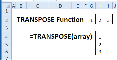
The TRANSPOSE function returns a horizontal range of cells as a vertical range, or vice versa.
How Could You Use TRANSPOSE?
The TRANSPOSE function can change the orientation of data, or be used with other functions:
- change horizontal data to vertical
- show total salary over best consecutive years
To change data orientation, without links,
- use Paste Special > Transpose.
TRANSPOSE Syntax
The TRANSPOSE function has the following syntax:
- TRANSPOSE(array)
- array is an array or a range of cells to be transposed
TRANSPOSE Traps
- TRANSPOSE must be entered as an array formula, by pressing Ctrl+Shift+Enter.
- The TRANSPOSE destination range must have the same number of rows and columns, respectively, as the array has columns and rows.
Example 1: Change Horizontal Data to Vertical
If data is arranged horizontally in a worksheet, you can use the TRANSPOSE function to list the data vertically, in a different location. For example, in a summary sheet, or dashboard, a vertical layout might be best. With the TRANSPOSE function, you could link to your original horizontal data, without changing its layout.
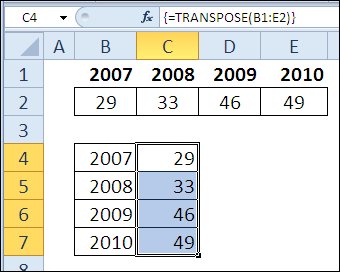
To transpose a 2 row x 4 column horizontal range to a 4 row x 2 column vertical range:
- Select the 8 cells where you want to display the data vertically — cells B4:C7 in this example.
- Type this formula, then enter it as an array formula, by pressing Ctrl+Shift+Enter.
=TRANSPOSE(B1:E2)
Curly brackets will be automatically added at the start and end of the formula, to show that it is array entered.
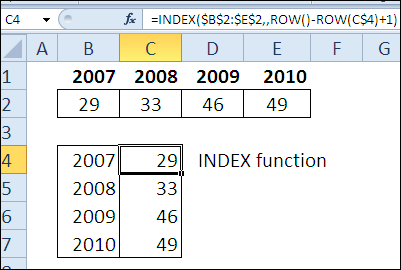
Instead of using TRANSPOSE, you could use another formula to display the data, such as this INDEX formula. It does not require array entry, and you don’t have to select all the destination cells when creating the formula.
=INDEX($B$2:$E$2,,ROW()-ROW(C$4)+1)
Example 2: Change Orientation Without Links
If you just want to change the orientation of your data, without keeping a link to the original data, you can use Paste Special:
- Select the original data and copy it
- Select the top left cell of the destination range
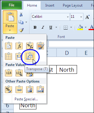
- On the Ribbon’s Home tab, click the Paste drop down arrow
- Click Transpose
- (optional) Delete the original data.
Example 3: Total Salary For Best Consecutive Years
The TRANSPOSE function can be used with other functions, as in this eye-popping formula. It was posted by Harlan Grove, in the Excel newsgroups, in a discussion on calculating the total salary for best 5 consecutive years.
=MAX(MMULT(A8:J8,–(ABS(TRANSPOSE(COLUMN(A8:J8))
-COLUMN(OFFSET(A8:J8,0,0,1,COLUMNS(A8:J8)-Number+1))
-(Number-1)/2)<Number/2)))
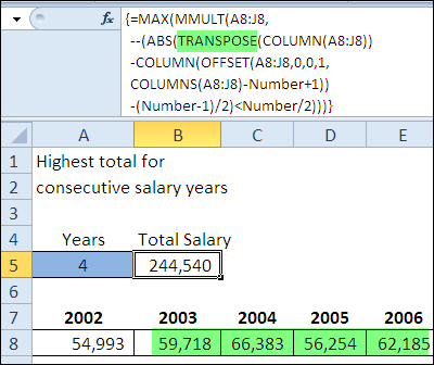
As you can see by the curly brackets in the formula bar, this formula is array entered. Cell A5 is named Number, and I’ve entered 4, for the number of years this example.
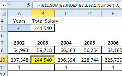
The formula tests the ranges to see if there are enough consecutive COLUMNS. The results of those test (1 or 0) are multiplied by the cell values, to get the total salaries.
To check the results, in the rows below the salaries, the total salaries for each starting cell are shown, with the maximum value highlighted in yellow. This is a long way to accomplish what the previous formula did in one cell!
Download the TRANSPOSE Function File
To see the formulas used in today’s examples, you can download the TRANSPOSE function sample workbook. The file is zipped, and is in Excel 2007 file format.
Watch the TRANSPOSE Video
To see a demonstration of the examples in the TRANSPOSE function sample workbook, watch this short Excel video tutorial.
_____________

Not to mention that for some matrix or vector calculations it is necessary to transpose a column vector to a row vector or vice versa. matrix multiplication (MMult) is one.
Or that multiplying a row vector (a,b,c) with a row vector (1,2,3) results in a row of results (a*1,b*2,c*3) but multiplying a row vector (a,b,c) with a column vector (1;2;3) results in a matrix of results (a*1,b*1,c*1;a*2,b*2,c*2;a*3,b*3,c*3)
we’re not all financial modelers.
Though we’re dealing exclusively with Transpose as a Worksheet Function it’s worth mentioning also that Transpose is handy working with VBA Arrays
See below for quick (much simplified example) of how to concatenate a vertical vector into a single delimited string – no loops etc…
Sub Example()
MsgBox Join([TRANSPOSE(A1:A10)],”,”])
End Sub
Transpose here converts the 2d Array (1 by n, 1 to 1) to a 1d Array (1 by n) allowing us to utilise Join.
(we need not utilise Transpose via Evaluate but in the context of the Worksheet Function it makes sense)
Apologies if this is way off track…
@ikkeman
Here here!
If you understand matrix math you can do quite a lot with Excel. I use it to define names using formulas and create graphs. It really minimizes the size of the spreadsheet – 20 to 30 kb instead of 20 to 30 Mb.
The last two times I needed to rearrange a significant amount of data, I used the INDIRECT function.
I worked through this formula from Example01: =INDEX($B$2:$E$2,,ROW()-ROW(C$4)+1) That works well. I expanded the array to include the years in Row 1, so $B:$1:$E:2. Then I included 1>4 in the row argument, teaching myself also the index and row functions as well. Good and thanks.
Re Example02… I did something similar recently at work. I did COPY…PASTE SPECIAL…PASTE FORMULAS…TRANSPOSE…OK. This took my table I’d already built and transposed it which I then used as source data for chart. Worked great.
Re Ex01, the fact you have to select your destination range before you enter your array formula can be a deal-killer on large ranges. Agree?
@Art, yes that makes it difficult to use the TRANSPOSE function with large ranges.