You can use the SUBTOTAL function to count visible items in a filtered list. In today’s example, AlexJ shows how to count the unique visible items in a filtered list. So, if an item appears more than once in the filtered results, it would only be counted once. Thanks, AlexJ!
Count the Unique Items
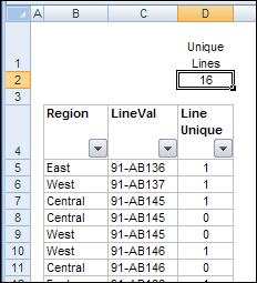
In the screenshot below, the formula in column D shows a 1 for the first instance of each item, and a 0 for all subsequent instances. For example, in cell D7, there’s a 1, counting item 91-AB145, and in the next two rows the count for the same item is zero.
The formula in cell D5 is:
=(COUNTIF($C$5:$C5,$C5)<2)*1
Apply a Filter
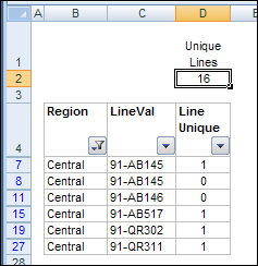
However, when the list is filtered to show only the Central region items, the total in cell D2 still shows 16 unique items, and cell D11 shows a zero for item 91-AB146, even though it’s the first visible instance of that item.
To solve the problem, AlexJ added some helper columns to the table. First, in column E, he created a formula to check if the row is visible. The formula in cell E5 is:
=1*SUBTOTAL(3,$D5)
AlexJ uses the 1 multiplier at the start of the formula to avoid the problem of the last row not being included in the AutoFilter range.
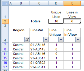
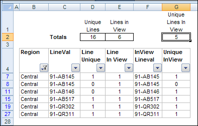
Based on this new formula, the total in cell E2 correctly shows that only 6 rows are visible.
Test For Visible Rows
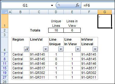
Next, in column F, AlexJ created a formula to show the item name if the row is visible. For hidden rows, the formula displays a hyphen instead of the item name. In cell F5, the formula is:
=IF($E5,$C5,”-“)
In cell G1, I tested the result for hidden cell F6, and you can see the result is a hyphen.
Count Unique Visible Items
Finally, in column G, AlexJ created a formula to check for unique items in column F, where only the visible rows have an item name. In cell G5, the formula is:
=($F5<>”-“)*(COUNTIF($F$5:$F5,$F5)<2)
With this formula, the hidden rows are ignored, and the count of unique items in cell G2 is correct for the filtered rows. The item 91-AB145 is counted only once, even though it’s in the filtered results twice, and item 91-AB146 is counted, even though it’s not the first instance of that item in the full list.
Array Formula to Count Unique
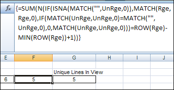
Another way to count unique items in a filtered list, is with named ranges and an array formula, as described in the July 2001 issue of Excel Experts E-letter (EEE). That formula is in cell F3 below, and shows the same results as AlexJ’s formula in cell G3.
Make sure you do a few warm up stretches before you attempt this one!
Download the Sample File
To see AlexJ’s formulas, you can download Alex’s sample file from the Contextures website.
On the AlexJ Sample Files page, go to the Filters section, and look for: FL0001 – Count Unique Items in Filtered List
_______________

I have a problem guys and i need to sort it out just by todays end or i land in a problem.
Hi
i have written the following code , which searchs through various columns and basically filters my data and then copies it to another worksheet, but i am facing one problem, the source data has a column containing hyperlinks to various other files on the system, but the copied data does not copy the hyperlink, i have to give a presentation at my college and need to sort this problem out by today afternoon, please help me out with the same.
The code is ‘
Option Explicit
Private Sub Worksheet_Change(ByVal Target As Range)
Dim rngCrit As Range
Set rngCrit = wksCrit.Range(“CriteriaRng”)
Application.EnableEvents = False
Select Case Target.Address
Case Range(“SelReg”).Address
rngCrit.Cells(2, 1).Value = Target.Value
Case Range(“Selcountry”).Address
rngCrit.Cells(2, 2).Value = Target.Value
Case Range(“SelCount”).Address
rngCrit.Cells(2, 3).Value = Target.Value
Case Range(“SelCity”).Address
rngCrit.Cells(2, 4).Value = Target.Value
Case Range(“SelDate”).Address
rngCrit.Cells(2, 5).Value = Target.Value
Case Range(“WhHotN”).Address
rngCrit.Cells(2, 6).Value = Target.Value
Case Range(“WhResN”).Address
rngCrit.Cells(2, 7).Value = Target.Value
Case Range(“WhOffN”).Address
rngCrit.Cells(2, 8).Value = Target.Value
Case Range(“WhRetN”).Address
rngCrit.Cells(2, 9).Value = Target.Value
End Select
If Range(“SelReg”).Value = “” Then
rngCrit.Cells(2, 1).ClearContents
End If
If Range(“Selcountry”).Value = “” Then
rngCrit.Cells(2, 2).ClearContents
End If
If Range(“SelCount”).Value = “” Then
rngCrit.Cells(2, 3).ClearContents
End If
If Range(“SelCity”).Value = “” Then
rngCrit.Cells(2, 4).ClearContents
End If
If Range(“SelDate”).Value = “” Then
rngCrit.Cells(2, 5).ClearContents
End If
If Range(“WhHotN”).Value = “” Then
rngCrit.Cells(2, 6).ClearContents
End If
If Range(“WhResN”).Value = “” Then
rngCrit.Cells(2, 7).ClearContents
End If
If Range(“WhOffN”).Value = “” Then
rngCrit.Cells(2, 8).ClearContents
End If
If Range(“WhRetN”).Value = “” Then
rngCrit.Cells(2, 9).ClearContents
End If
If Not rngCrit Is Nothing Then
wksResRep.Range(“B1:W65?).AdvancedFilter _
Action:=xlFilterCopy, _
CriteriaRange:=rngCrit, _
CopyToRange:=Range(“ExtractDetails”), Unique:=False
End If
exitHandler:
Application.EnableEvents = True
Exit Sub
errHandler:
Resume exitHandler
End Sub
Please reply back soon.
Thanks
Wonderful work. I am surprised that there isn’t a subtotal function that exists in Excel to handle this calculation. I’m very impressed and am excited that such a niche need was fulfilled…great site! I’m now a new fan!
I found this on another website. I don’t ubnderstand it, but it works and no need for extra helper cells:
=SUM(IF(FREQUENCY(IF(SUBTOTAL(3,OFFSET(A2:A100,ROW(A2:A100)-ROW(A2),0,1)),MATCH(“~”&A2:A100,A2:A100&””,0)),ROW(A2:A100)-ROW(A2)+1),1))
…be sure to hit CONTROL+SHIFT+ENTER after pasting this formula. This is for a range of A2:A100, adjust the range accordingly.
Source:
http://www.mrexcel.com/forum/excel-questions/395996-count-unique-values-filtered-list.html
(see 3rd comment down)
123456
Exmple:
i have write some text in only one cell so can I count this?
which text type in only one cell….
Please answer