You can use data validation to create drop down lists in Excel. With a bit of Excel magic, you can create dependent drop down lists, so the selection in one drop down controls what appears in the next drop down. You’ll see different drop down lists in the same cell!
We’ll take a quick look at how a basic dependent drop down works, then add flexibility by changing the data validation formula.
Select Countries and Cities
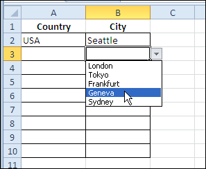
For example, in the worksheet shown below, there’s a drop down to select a country in column A. If you select USA as the country, cities from the USA appear in the Column B drop down.
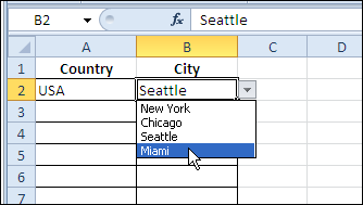
This is created by using the INDIRECT function in the data validation settings for column B:
=INDIRECT(A2)
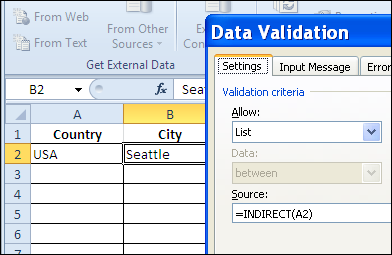
There are city lists in the workbook, and each list is named to match its country name. So, if you select USA in cell A2, the INDIRECT function references the range named USA.
Change the Formula
Currently, the drop down list in column B doesn’t work, unless you first select a country in column A. We’d like to give users the option to select a world city, if they haven’t selected a country in column A.
On the Lists worksheet, there’s a range named World, highlighted in the screen shot below.
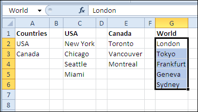
Just as you can use the IF function on the worksheet, you can use it in a data validation formula. For the data validation cells in column B, we’ll change the formula to the following:
=IF(A2=””,World,INDIRECT(A2))
If cell A2 is blank (equal to an empty string “”), then show the World list. Otherwise, show the list for the country selected in cell A2.
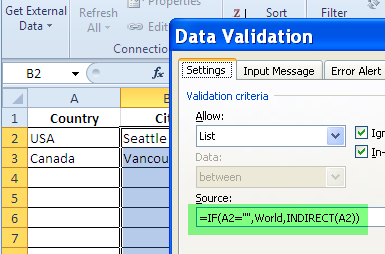
After this change to the data validation formula, if you click on a drop down arrow in column B, and no country is selected in column A, the list of world cities appears.
Watch the Video
To see the steps for creating a basic dependent drop down list, then adding an IF function, watch this Dependent Data Validation video tutorial.
________________

This is partly what I have been looking for. What I need is a way of automatically inserting a value in a cell, which is dependant on the adjacent cell. EG in cell A2, I would enter a value from a drop down list (list defined as ‘ORG’ on my LookUp sheet), then in cell B2, would automatically show the corrseponding code for the entry in A2 (list of codes defined as ‘COD’ on the LookUp sheet.) I am struggling a little.
Tony-
You need to create a defined name that includes both ORG and COD on your LookUp sheet. For example, if ORG is in A1:A10 and COD is in B1:B10, create another name called, say “ORGCOD”, that represents A1:B10.
Then use this in B2 on the main sheet:
=VLOOKUP(A2,ORGCOD,2,0)
Cheers Jason. Will give this a try. Thought VLOOKUP might have been the answer, but was not sure how to go about it. Many thanks.
Hi Jason. Worked at treat, with a little tweaking. I used the simpler LOOKUP function with an error trap (always struggle with the IsError function):
=IF(A2=””,” “,(LOOKUP(A2,ORGCOD,COD))
Thanks for pointing me in the right direction.
Tony,
Just a word of caution with LOOKUP. Your ORG dataset (what Excel Help calls “lookup_vector”) has to be in ascending order or your formula may return a wrong value. My other issue with LOOKUP is that if doesn’t find an exact match, it will select the largest value less than your lookup_value (which may be OK in your situation).
All of this is well-documented in the Excel help file, so take a look.
Knowing this, I always use VLOOKUP and specify exact match (use 0 in 4th argument). In my analyses I always want an exact match and if VLOOKUP can’t find one, then I want to see #N/A.
Very elegant solution.
This is one of the proofs that dynamic process-driven approach to data in Excel(ver. data driven) is absolutely possible.
Thank you for sharing
I’ve always struggled to find a good reason to use the INDIRECT function. You’ve not only solved this problem for me, but shown a great trick for drop-down lists. Good stuff.
[…] For detailed instructions see Different Drop Down Lists in Same Excel Cell […]
Debra, many thanks for sharing this! I’ve been looking for a solution exactly as you have shown, and I didn’t know the INDIRECT function. Your post really helped me!
Hi, thanks for your nice post.
Is it possible to allow multiple selections in one cell ? (in your example it should be possible to select multiple cities).
Thanks in advance for your help.
Hi everyone,
I have a real conundrum here. I am trying to create a form which uses drop downs and vlookups but I have hit a brick wall when trying to achieve the following. Can anyone assist please?
I have a drop down which has values such as “Support Staff Outer – 7 – £10000″,”Support Staff Outer – 8 – £20000” and “Teacher Main – 1 – “19539” and so on. I want the next drop down to look up changeable partial text string within the first drop down (eg *Support Staff Main* or *Teacher Main*) and return all table values as another drop down.
My Initial Drop down has the following values
Support Staff Main – 1 – £12266
Support Staff Main – 2 – £12435
Support Staff Main – 3 – £12614
Support Staff Main – 4 – £12915
Support Staff Main – 5 – £13321
Support Staff Outer – 1 – £14844
Support Staff Outer – 2 – £14962
Support Staff Outer – 3 – £15089
Support Staff Outer – 4 – £15368
Support Staff Outer – 5 – £15771
Teacher Main – 1 – £21804
Teacher Main – 2 – £23528
Teacher Main – 3 – £25420
Teacher Main – 4 – £27376
Teacher Main – 5 – £29533
On a separate worksheet sheet I then have a table with these values
Column A
Support Staff Main
Support Staff Main
Support Staff Main
Support Staff Main
Support Staff Main
Support Staff Outer
Support Staff Outer
Support Staff Outer
Support Staff Outer
Support Staff Outer
Teacher Main
Teacher Main
Teacher Main
Teacher Main
Teacher Main
Column B
Support Staff Main – 1 – £12266
Support Staff Main – 2 – £12435
Support Staff Main – 3 – £12614
Support Staff Main – 4 – £12915
Support Staff Main – 5 – £13321
Support Staff Outer – 1 – £14844
Support Staff Outer – 2 – £14962
Support Staff Outer – 3 – £15089
Support Staff Outer – 4 – £15368
Support Staff Outer – 5 – £15771
Teacher Main – 1 – £21804
Teacher Main – 2 – £23528
Teacher Main – 3 – £25420
Teacher Main – 4 – £27376
Teacher Main – 5 – £29533
The formula in the validation would need to be dynamic so that if I drop down “Teacher Main – 3 – £25420” in the first drop down that it would look to the table and return all of the values listed against the table column A equal to “Teacher Main” and return the column B values linked to that in the second drop down. Or if I was to drop down the value of “Support Staff Outer – 3 – £15089” in the first drop down then the second drop down would show values linked to “Support Staff Outer” in the table. Is this possible?
Is it possible to have multiple drop down box in same cell?
because what i really want to happen is like
in the same cell, this is how it would look like
(dropdownlist)-(dropdownlist)-(dropdownlist)
3 dropdown box in one cell.. is this possible?
I Have new scenario,
sheet1
Column A Column B
ABC 1
ABC 2
ABC 3
ABC 4
DFG 5
DFG 6
DFG 7
DFG 8
Now in sheet2
Column A
IF
ABC is selected in dropdown list then only the number which are in front of ABC should be displayed in a new dropdown list.
@Piyush, you could use the dependent drop down technique shown here:
http://www.contextures.com/xlDataVal13.html
I have a problem with the basic Indirect validation function! With the example, I have used labelling of the Source data for validation to bring up the drop down list “USA, Canada” etc and then having labelled the other columns as per the city they refer to, used the =INDIRECT(A2) in data validation under “list” to reference the country and bring up the cities. The problem is, the list being shown under cities is still countries – i.e. the source list is simply being repeated and the two lists appear to have no dependency! Why do you think this is happening? I have followed the instructions to the letter!
Please help – I have to get this nailed by Monday next week! Thank you 🙂
What is selected from the drop down list in cell A2? Is it a country name, e.g. USA?
If you check the Name Manager, is there a workbook level name that matches that selection?
Check the address in the Name Manager’s Refers To box for that name — then, go to that range and check the contents.
Something is wrong somewhere!
Thank you for the great, easy to follow tutorials.
I’ve learned a lot through your blog and I can highly recommend it to friends 🙂
On a side-note.
For a while the IF-statement had me stumped. It would create an error, everytime I inserted in one of my worksheets.
On both Excel for Mac 2010 and Office 2010.
As it turned out, those versions don’t accept the ‘,’ as seperator. Instead you need to use ‘;’ 😉
Other than that, flaweless tutorials. The only ones I could find, that have learned me so much about Excel 😀
Thanks a million!
Greetings,
Bran
It is really mind-blowing.
can we do the same in google sheets? if yes please guide me how to do.