
This week I’m working on a client’s sales plans for the upcoming fiscal year. They forecast sales per month by product and customer, and we use some pretty complicated formulas to sort things out. Of course, anywhere that it makes sense to use a pivot table, I create one. It’s a great way to summarize all the details, and review the overall totals. Running totals are easy with Excel pivot tables!
No Formulas for Pivot Tables
For example, on a worksheet you can use formulas to create a running total, but in a pivot table it’s much easier — you can quickly create running totals with a couple of mouse clicks.
Let’s take a look at an Excel pivot table based on some faked sales data. In the screen shot below, you can see the total sales per region per month, and the Grand Total per month. By changing the Sales field settings, you can show a running total, instead of the normal Sum.

Add the Running Total
To change the sales field, and show a running total, follow these steps:
-
- In the pivot table, right-click one of the Sales amount cells.
- In the context menu that appears, click Summarize Data By
- Click More Options

-
- In the Value Field Settings dialog box, click the Show Values As tab
- From the Show Values As dropdown list, select Running Total In.
- Select the Base Field where you want to see the running total. In this example, we’d like to see the running total down the list of dates, so OrderDate is selected as the Base Field.

- Click OK, to close the Value Field Settings dialog box.
The pivot table changes, to show the running total for sales.
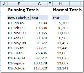
In the following screenshot, you can see the running totals in column C, and the original monthly totals in column H. Each month’s total sales is added to the previous total, to show the running total.
Change the Running Total Base Field
The most common use for running totals is to show amounts accumulated over time, as in the sales by month example above. However, you can use a non-date field as the base field for a running total. For example, in an election, you could show a running total of votes as each district submits its results. Or, for a large construction project, you could show a running total of expenses over the project phases.
In this pivot table, I’ve added City to the Column area, and used that as the Base Field for the running total.

Now, instead of the running total going down the pivot table by month, it goes across the pivot table, by city.
Be careful though — if you use a Base Field that isn’t in the pivot table layout, you’ll see #N/A for all the running total values.

Running Totals Stop at Year End
If your pivot table shows the data grouped by year and month, the running total will stop at the year end, then start over for the next year. For a workaround, there are instructions on my pivot table blog:
http://www.pivot-table.com/2013/07/17/running-total-stops-at-year-end/
Running Totals in Excel 2003 Pivot Tables
The running total technique is similar in Excel 2003 pivot table, and you can see the instructions here: Excel 2003 Pivot Table Running Totals. It also shows the results when there are multiple fields in the row area, and a running total is added to one of those fields.
Watch the Running Totals Video
To see the steps for creating running totals in Excel 2003, please watch this short Pivot Table Running Totals video.
__________
Great article. I have been certain that this feature must have been within Excel somewehre but not found it until now. Just a shame it has taken me so long…..time for some more analysis with Excel…..
Mike
I enjoyed reading this excellent article: it gave examples of applications, it was easy to follow the technical details and it gave examples of mistakes to avoid. The video cleared my unease about the Base Field. Q1 How would I do a running total where the running total is decreasing? My application is an inventory. My data is date versus number of a product sold on that date. I want date versus decreasing stock level for that product on that date.
Example of what I have:
Date Count #
15/01/13 100
16/01/13 1
17/01/13 7
18/01/13 1
Example of what I would like:
Date Stock level in warehouse
15/01/13 100
16/01/13 99
17/01/13 92
18/01/13 91
Kind rgds Goronwy Glyn Price
Hi There
I have a pivot chart where I have created a running total of expenditure over a date field – my problem is that this expenditure runs over numerous years. The pivot chart zeros the running total at the end of each year and starts in January from zero again. I there fore have a running total per year but not over years – can you help?
Regards JOHN
Hi John,
Did you find any solution?
I have the same issue which you have.
Do let me know if you can help me too
Did you ever figure this out? I too, have figures by quarter and by year (two separate fields). I do not want the running total to reset at the start of each year, but I also want to be able to show the data by quarter.
@Scott, there are instructions on my pivot table blog:
http://www.pivot-table.com/2013/07/17/running-total-stops-at-year-end/
Instead of year-month, you could create column with year-quarter, then base the running total on that field.
Nice! I was developing a SSAS cube and found this extremely helpful to calculate the running totals in the pivot table. I orginally put a calculated member into the cube and had to write some MDX. Thanks!!!
My problem with using running totals in PivotCharts is I want the running total to STOP when there are no more additions. Instead, a horizontal keeps going at the point where the total left off. I would have everything I need if there were an option to stop the progression if the line stays horizontal.
Hi Josh, did you find the solution on your problem? I have the same problem and I don’t know to solve it…
To get the inventory count decreasing over time (a decreasing running total):
– multiply the number sold by -1
– then put the answer to this in the running total field
so;
A : B : C
day1:100:100
day2: 1: -1
day3: 2: -2
day4: 1: -1
then put colC in the pivot table and do a running total with base field colA
how to make copy of running balance in excel 2013 to other worksheet
Thanks for the nice article . It helped me.
Hi, I have a question about this topic.
I have some amounts in one column, and this amounts represent a batch process. Therefore, in one moment (periodically) this amount is 0 (when a new batch starts because the previous one is full) and it starts to increase again. So I want the cumulative sum but in the moment in that the amount is 0, the cumulative sum should start from 0. At this moment, I have only found the formula which does the cumulative sum, but I don’t know how to “reset” the cumulative sum in the moment that the amount is 0. I would be so grateful if you could help me. Thank you.
Always enjoy your well presented explanations, although I have to listen to or read several times for it to “sink in.” Smile. First, for FYI, the video and the written instructions are for different versions of Excel, at least I think? Second, probably 99.99998% of what I’ve read on the Internet about calculating running totals does not even come close to describing what I shall refer to as a “continuous running total” for a specified time period, e.g. 12 months, not 13 but 12. For example, you have some amounts entered for each month, Jan through Dec. When you enter an amount for the next month, i.e., Jan, the running total will be Feb of the previous year though Jan of the current year, i.e., 12 months. You may have discussed this already – sure hope so!! Might you point me in the right direct Debra? As always, you are most thoughtful and considerate and an excellent teacher! Best upcoming Holiday Wishes to you and your family. Mort in Dallas
Hi Mort,
I included the Excel 2003 video, because lots of people were still using that version, when I wrote this article. The main instructions and screen shots are for Excel 2010.
If you want to do a rolling 12 month total in a worksheet table, you could use SUMIF. Assuming the list is sorted by date, with dates in column A, and amounts in column B, use this formula:
=SUMIF(A$2:A2,”>=” & DATE(YEAR(A2),MONTH(A2)-11,DAY(A2)),B$2:B2)
Hi All,
Apologies if this thread has already been answered. I want to stop showing cumulative graph when there is no new data. I have zero values as the dates have not been realized this shows up as flatspot on the graph. Is there any way to stop the pivot chart plotting the zero values.
Thanks in Addvance
Hi, know this is an old thread, but maybe someone can help. What I’ve been counting is the number of years someone stays active in a program. I want to show a graph that starts with the total number and subtracts the count of everyone who left after one year, two years, etc. Any ideas on this?
Thank You!