For the past 82 years (approximately), I’ve used Excel almost every day. Along the way, I’ve learned a few tricks, and produced some sophisticated workbooks.
One of the joys of Excel is that there’s always something new to learn. And this week I learned how to freeze panes to hide rows in Excel.
Too Many Heading Rows
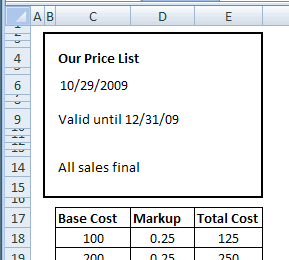
This week, while working on a client’s files, I wanted to review some calculations in a price list. The top 15 rows are headings for the printed sheet, then there’s a row of column headings for the price calculations.
Below that are hundreds of rows with prices. Here’s a simplified version of the worksheet.

A Frozen Wasteland
I wanted to see those column headings, and as much of the price list as possible. However, if I selected row 18, and froze the worksheet, I’d be stuck with a couple of inches of wasted space, with all the headings visible at the top.
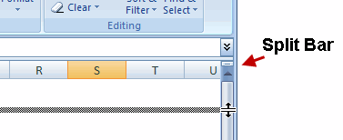
Instead of freezing, I could drag the split bar down, to split the screen, and create a small section at the top. Next, I could scroll the column headings into view in the top section of the screen.

A Splitting Headache
I’m not sure why, but I don’t use split windows too often.
Anyway, as I played with the scroll bar, and thought about splitting the window, I accidentally froze the panes. (Trust me, it’s easier to do that in Excel 2003 than in Excel 2007.)
When this happened, row 17 was at the top of the window, and row 18 was selected.
First Visible Row Frozen at Top
Miraculously, row 17 was frozen at the top of the screen, and all the rows above it were out of sight.
So, instead of wasting 2 inches of space, only 1/4 inch was used, and I could see more of the price list.
Why didn’t I know about that before? Or maybe I did know it, many years ago (or last week), and forgot about it.

A Warning for You
The only downside to this Freeze Panes trick is that my client might not notice the Freeze Panes line above row 18.
That thin line can be hard to see, especially if the worksheet gridlines are showing.

Confusing Worksheet Situation
If people don’t notice the Freeze Panes line, they might think that the first 16 rows have been hidden.
And, if they try to show those row again, by using the Unhide command, it won’t work.
Also, if they click anywhere on row 17, and try to scroll up, nothing will happen. Scrolling doesn’t work in the frozen part of the screen.
So, if you use this trick to temporarily hide rows, remember to unfreeze when you’re finished working. Be kind to your co-workers (or clients)!
What Did You Learn About Excel?
So that’s my new trick. What did you learn about Excel this week?
Something less embarrassing than my lesson, I hope!
Freeze Panes to Hide Rows in Excel

________

> For the past 82 years (approximately)
Debra is getting dyslexic. She has, of course, been using Excel for 28 years – since she was 2.
Thanks for the support Ed! Too bad I can’t remember exactly when I started using Excel. It must have been around 1989/90.
When I have too many rows on top of the freeze pane, I like to group some (e.g. rows 1:16 in your example) so I can quickly switch back and forth.
Thanks Sébastien, that’s a good use of the grouping feature.
You can do a similar trick in the VB editor as well. Each code window has that same “Split Bar” (the small rectangle at the top of the vertical scroll bar)… you can drag it down to split the code window into two separate parts, each independently scrollable. And you can do this for both the Procedure View or the Full Module View (those two icons down in the bottom left corner of each code window). In Full View, each window has all the procedures “scrollably” available all the time; in Procedure View, you have to select the procedure individually for each of the split-window views. I find splitting the code window this way quite handy when trying coordinate the code between two related procedures during development.
Thanks Rick, that’s great advice on using the VB editor windows effectively.
Just to be clear, i take it that instead of freezing row 17 at the time when you could also see rows 1 – 16 (i.e. you were scrolled to the top), you scrolled down the worksheet until row 17 was at the top, and thent freezed panes?
I.e. scroll first, freeze later.
Jeff, that’s right, and thanks for asking for clarification. I added a sentence to the article to make the steps clearer.
Your article reminded me of some of my most frustrating times in Excel… when someone froze the panes while using filters, then cleared the filters but never unfroze the panes. There I am going up and down and left and right with the arrow keys, but NOTHING is happening on the screen. Fortunately (sort of), it’s happened to me enough times so now I know it’s related to freeze panes.
Bob R, I don’t recall running into that problem (yet!), so thanks for the warning.
Dear Debra,
What a great idea for a new blog, the Excel Serendipity blog, where people share what they learnt.
I had three such happenings in the last few days. One was a horror story, the second a “Wow” moment and the third a lesson well learnt.
The horror story comcerns DATES, MACROs and EXCEL
i have a column of text formatted dates that come form our ERP system
05.07.1998
when i amnually replace the . with a slash i correctly get 5/07/1998,
HOWEVER, when i perform the same operation via VBA i get 7/05/1998 and for my purposes this is incorrect.
I solved the problem in a convoluted way by writing the following code:
dot1 = InStr(1, x, “/”, 1)
dot2 = InStr(InStr(1, x, “/”, 1) + 1, x, “/”, 1)
xDay = Mid(x, 1, dot1 – 1)
xMonth = Mid(x, dot1 + 1, dot2 – dot1 – 1)
xYear = Mid(x, dot2 + 1, Len(x) – dot2)
newdate = xDay & “/” & xMonth & “/” & xYear
Range(Cells(r1, c1), Cells(r1, c1)).Value = CDate(newdate)
Range(Cells(r1, c1), Cells(r1, c1)).NumberFormat = “dd/mm/yyyy”
Where x is the text string. Thankfully this works.
Happy discovery was the following =TEXT(A1,”dddd”) returns the day of the week for a given date.
Learning for the week was thanks to the BRILLIANT paper on SUMPRODUCT on the XLDYNAMICS.com website. Now understand why “*” was required, also learnt that with “–” you do not need “*” in in SUMPRODUCT
Kanti, thanks for sharing your Excel experiences from the past few days. I’m glad the horror story turned out okay in the end. 😉
Kanti,
Assuming the variable x contains your date value with the “dot” delimiter, these three lines of code should do exactly what your posted code does…
Parts = Split(x, “.”)
Cells(r1, c1).Value = DateSerial(Parts(2), Parts(1), Parts(0))
Cells(r1, c1).NumberFormat = “dd/mm/yyyy”
Note that I assumed your Range(Cells(r1,c1),Cells(r1,c1)) reference was meant as a reference to a single cell… that construction is identical to Cells(r1,c1), which is what I used in my code above. You might want to look up the Split and DateSerial functions in the help files to better understand what my code is doing.
Dear Rick,
Thanks for your input, i will certainly try your suggestion. So much to learn so little time.
regards
kanti