Instead of showing all the data in a chart, you can select a specific date range, and show only the data from that period. In this example, drop down lists of dates are created with data validation. Select Excel chart dates from a drop down list, and the chart changes to show the new range.
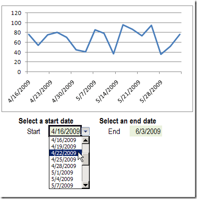
To create this dynamic chart in Excel 2007, you can create a table from the chart data, then create named ranges, and use those names in the chart.
Create an Excel Table for the Chart Data
[Note: Please see the post, Problems With Dynamic Charts in Excel and ignore this step — the Excel Table may cause problems.]
- On the Chart sheet, select a cell in the chart data, e.g. cell A1
- On the Ribbon, click the Insert tab, then click Table
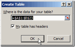
- In the Create Table dialog box, click OK, to create the table for the selected range.
Name the Start Date and End Date cells
- On the Chart sheet, select the Start Date cell (F17)
- In the Name box, type StartDate then press Enter, to name the cell
- Select the End Date cell I17, and in the Name Box type EndDate, then press Enter

Name the Chart Date Range
[Note: Because you did not create an Excel Table, as advised above, use the following formula in step 3, to create a dynamic range for the ChartDates:
=OFFSET(Chart!$A$1,1,0,COUNT(Chart!$A:$A),1)
- On the Ribbon, click the Formulas tab, then click Define Name
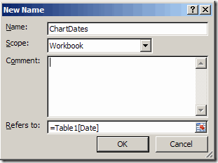
- Type ChartDates as the name for the range
- Click in the Refers To box, and select the Chart Dates (A2:A23) on the worksheet.
Because this range is in an Excel Table, the reference will automatically change to show the
table name and column name, Table1[Date] - Click OK
Create the Start Date and End Date dropdowns
- On the Chart sheet, select the Start Date cell (F17)
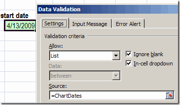
- On the Ribbon, click the Data tab, then click Data Validation
- From the Allow dropdown, select List
- In the Formula box type: =ChartDates
- Click OK, then repeat these steps to create a dropdown for the End Date.
Define the named ranges for X and Y values:
- On the Ribbon, click the Formulas tab, then click Define Name
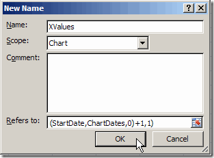
- Type a name for the series: XValues
- From the Scope dropdown, select the data sheet name, Chart
- Type a formula that finds the start and end dates in the data:
=OFFSET(Chart!$A$2,MATCH(StartDate,ChartDates,0)-1,0,
MATCH(EndDate,ChartDates,0)-
MATCH(StartDate,ChartDates,0)+1,1) - Click OK
- Follow the same steps to define the YValues named range, using the following Settings:
Name: Yvalues
Scope: Chart
Refers To: =OFFSET(Chart!XValues,0,1)
Create the chart
- Select a cell in the chart data
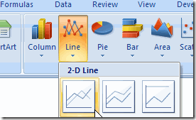
- On the Ribbon, click Insert, then click Line in the Charts group
- Click the first Line chart option
- To hide the Legend, click the Ribbon’s Layout tab, click Legend, and click None
Make the chart dynamic
- Select the chart, and click the line to select it
- In the formula bar, change the series formula, replacing cell references with range names:
=SERIES(Chart!$B$1,Chart!XValues,Chart!YValues,1)

Test the chart
- Select a start and end date from the drop down lists, and the chart will display that range
Warning: If you select the entire range, the series formula will revert to
absolute cell references instead of the named ranges. (This doesn’t happen in earlier versions of Excel.)
Download the Sample File
You can download the completed Excel 2007 sample file for Dynamic Date Range Charts.
[Note: Please see the post, Problems With Dynamic Charts in Excel and download that sample file — the Excel Table may cause problems.]
_________________

Can you not accomplish the same thing by filtering data in the table, ie., create table, use table to create chart and then filter data in table to dynamically change plotted data?
Sridhar, yes, you could use a filter to change the data that’s visible in the chart.
With the technique described here, you could store the data on a hidden sheet, protected from users, and give them access to the chart only.
[…] My colleague and fellow MVP Debra Dalgleish shows a dynamic chart approach that lets you Select Excel Chart Dates From a Drop Down List. […]
How woud you ensure that the end date is always greater than the start date?
You could use a formula to show a warning on the worksheet, e.g.
=IF(StartDate>EndDate,”Please select an end date after the start date”,””)
Or, use dynamic validation lists or programming to ensure that users don’t pick an invalid date.
The only issue with generating a warning with a formula is that it will still allow you to select an invalid value (end < start). Once that selection is made, the chart breaks and Excel generates its own error message.
My suggestion would be to create named ranges for the Start and End Date, using the same offset technique as is used for XValues and YValues. The StartValues range would start at the beginning of the list and continue through the EndDate – 1. The EndValues rante would begin at Start Date + 1 and continue through the end of the list. That way, the list of valid end dates is updated any time a selection is made for either date.
Alternatively, have the start date and end date be replaced in the formulae with MIN(start date, end date) and MAX(start date, end date), ensuring that whichever is the greater is used as the end date. I assume the graph would just look silly if the two dates were the same, not broken.
Hi Debra. I love this blog, which I’ve just discovered and spent several late nights reading.
Question for you: I see in your instructions that when you define the named ranges for X and Y values, you set the scope at the sheet level (i.e. you select the data sheet name ‘Chart’.
Is there any specific reason to set this at worksheet level, as opposed to workbook level?
One advantage I can see of using worksheet vs workbook is that if you use the ‘select data’ dialog box to add the dynamic series, you can push F3 and choose the worksheet name from the ‘insert names’ dialog box without having to prefix it with a worksheet or workbook name. However, I realise you didn’t use this approach above – you just overtyped the sheetname and series name into the formula bar.
Another advantage may be that you want to have similar graphs on each worksheet, using the same named range to access different series.
I initially thought that if your name is defined at the Workbook level, then in order for the graph to accept the range name you must prefix the Name with the spreadsheet filename. But I’ve since found that you can prefix it with just a sheetname (any one will do) and excel will accept the reference. If you then use the ‘select data source’ to look at what happened, you see it replaced whichever sheet name you used with the workbook name.
How can you do to place more data series?
I couldn’t get it to work with the offset formula in the ChartDates named range. I did get it to work though by just using the range itself (A2:A19 in my case), without making the range a Table.
I am also keen to see it work on multiple data series if possible.
Figured out the extra series bit:
You just need to make an extra named range for each extra series and then change the OFFSET formula for each series to =OFFSET(Chart!XValues,0,n) where n=how many columns the data is away from the date column.
Now I just have to figure out how to make a drop down to choose which series I want in the graph.
Many thanks Debra,
Carl.
I already have a chart, with a lot of data; however, i want to select only specific time frame- and i think the drop down menu would be great – but i cannot seem to have it running?! Is there any other formula to call specific dates in chart?
btw; i have different sheets to combine, they are not on one sheet?!
Would like to add a second set of data into the same graph. Is this possible and how would I do it.
Could someone help me throw the last step? Can’t change the series selection for some reason.
I can get it to work when creating my own file, but I can’t get it to work in an existing file. I even then tried transferring data from my existing file to the file I got it to work in, and now that’s not working. I wish there was a bit more detail on each step explaining its purpose, might help to figure out how to solve when things go wrong!